Ellen Ehrhardt - Robert B. Jacobson - Aaron J. DeLonay
Adding River Bathymetry to Flood-Plain Topography for Surface Water Modeling of the Missouri River1
ABSTRACT
Modeling habitats of the channel and the flood plain of the Missouri River provides an improved understanding of how river management affects fish and wildlife habitat. Using digital water models, the spatial distribution of depth and velocity of flowing water can be represented, thereby allowing available habitat to be quantified under varying discharges. This information, in conjunction with data such as fish location, makes it possible to quantify the range of aquatic habitat selected by the fish and then to identify the discharges that provide the most habitat.
Two dimensional surface-water hydraulic models require elevation meshes of channel topography for computation. A high-resolution (5-m cell) digital elevation model (DEM) is available for the flood-plain reach we are studying, but newly collected bathymetric data must be merged with it to compile an elevation mesh for the entire river corridor, floodplain and channel. Furthermore, habitat rehabilitation activities and natural processes of erosion and deposition in the river corridor will alter bathymetry in the future, so the mesh will have to be updated frequently. Hence we need a simple and rapid method to calculate true elevations from data representing depths below water-surface datums that vary over time. We have developed a procedure to estimate water-elevation surfaces using a minimum of field-determined water-surface elevations and ARC/INFO’s cost-distance function. The cost-distance and elevation grids are combined with grids of bathymetric survey depths to yield a surface of the river bottom in topographic units (feet above mean sea level). Finally the bathymetric grid of the river bottom is merged with the flood plain grid to produce an elevation mesh for use in the surface-water hydraulic model, making habitat modeling possible. The purpose of this report is to describe the process of data manipulation required to produce the integrated DEM-bathymetry topographic mesh.
1
Any use of trade, product, or firm names is for descriptive purposes only and does not imply endorsement by the U.S. Government.
INTRODUCTION
Physical aquatic habitat is typically described as the combination of water depth, velocity, temperature, water chemistry, and substrate that provides living spaces for aquatic organisms (Gordon and others 1992). In riverine ecosystems, physical habitat varies on timescales of individual floods - as inundated area varies as well as on timescales of geomorphic change – as topographic contours are altered by erosion and deposition.
Aquatic habitats of the Missouri River have been substantially altered by river management that has changed the timing and magnitude of floods as well as the topographic contours that control how water is distributed. Prior to management, the Missouri River was a wide, shallow, braided river, with abundant sandbars and side channels. Annual floods inundated large areas of the flood plain. Mainstem reservoirs constructed as part of the Flood Control Act of 1944 changed the magnitude and timing of floods, and bank stabilization and navigation structures substantially narrowed and simplified the channel. Subsequent construction of agricultural levees on accreted land disconnected the flood plain from the river. These alterations have been cited as the cause of degradation of physical habitat and declines of native river-corridor species (Hesse 1989). Velocities of the present-day self-scouring navigation channel are four times the tolerances of most fish (USFWS 1980).
Mitigation efforts aimed at rehabilitating the Missouri River for native river fish such as the endangered pallid sturgeon, requires that critical fish habitat be identified and quantified. Remotely sensed data and spatial modeling are essential tools in this effort. Digital, two-dimensional surface-water hydraulic models can be used to map the spatial distribution of depth and velocity of water for a given discharge. Integrating the spatial distribution over time yields an understanding of when, how long, and how much of particular habitats are available (Waddle and others, 1997). This information, in conjunction with data such as fish location and habitat use, makes it possible to quantify the range of aquatic habitat selected by the fish and then to identify the discharges that provide the most critical habitat.
Life history research and critical habitat characterization assists biologists in making recommendations for timing and levels of river discharge, thus promoting the rehabilitation of habitats for native river fish and wildlife such as the pallid sturgeon, blue sucker, and least tern (DeLonay et al. Personal Communication, Dugger 1997, Tibbs 1995, Tibbs 1997). Quantification of habitat availability over time and space requires GIS tools for data collection, analysis, and presentation (for examples see Panfil and Jacobson, 1999, Waddle and others, 1997).
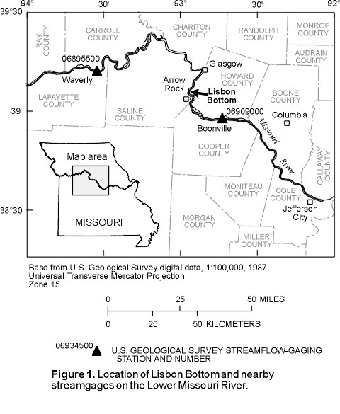
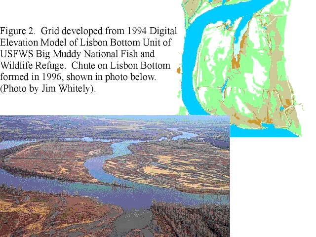
A topographic mesh is the fundamental data requirement for the surface-water hydraulic modeling. This paper describes the development of such a mesh for the Lisbon Bottoms Unit of the USFWS Big Muddy National Fish and Wildlife Refuge (Fig. 1). For this river reach, we have available a high-resolution, 5-m cell digital elevation model (DEM), constructed in 1994, for modeling flow over the flood plain. However, this DEM lacks channel bathymetry and does not include a large secondary chute that was eroded across the flood plain in 1996 (Fig. 2 ). Updated bathymetric data are collected using conventional hydrographic survey equipment on a small boat, using sub-meter differential GPS.
Depth is collected in relation to the water surface. However, the river water-surface elevation is sloping and the slope and depth change continuously with changing discharge. Over longer time intervals (years to decades) channel modifications due to engineering structures, habitat rehabilitation projects, or natural erosion and deposition, necessitate frequent updates of bathymetry to maintain habitat inventory models. To compile data acquired under a broad range of conditions, we require a simple and rapid method to define water-surface elevations, which can then be used to calculate true elevations from water depth data. The purpose of this report is to describe the process of data manipulation required to produce the integrated DEM--bathymetry topographic mesh.
METHODS
Development of a topographic mesh for Lisbon Bottom required integration of data from a 1994 DEM and bathymetry of the main channel and side channel. This integration was complicated by different reference frames of the data sets. The z-units of the landscape DEM were in units above sea level while the bathymetric data was measured as depths below the water surface. Since the water surface slopes in a downstream direction, a simple addition or subtraction procedure could not be used to convert depth data to true elevations. We overcame this obstacle using the COSTDISTANCE function of GRID.
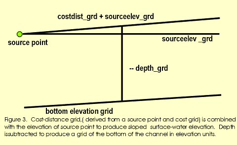
Development of the topographic mesh for surface-water hydraulic modeling of channel and flood plain features required first, construction of a representation of the sloped river surface in elevation units, secondly, integration of depth data from transects collected over several days and discharges and finally, integration of data from a 1994 digital elevation model (DEM) of the study area. The bathymetric data needed to be converted from depth based data (depth below the water surface) into the same elevation-based reference frame of the flood-plain DEM. The COSTDISTANCE function in GRID was used to model and distribute the slope or cost of moving up-river. The slope was added to the elevation of a starting point with a known elevation to model the surface-water elevation (feet above mean sea level). Depth was then subtracted from the water-surface grid to produce a grid of the topography of the channel bottom. The final grid was developed by merging the flood-plain grid with the bathymetry grid (Fig. 3 ).
Preparation of the Flood-plain DEMs
Component DEM panels were brought into ARC/INFO as floating point grids with the ARC command DEMLATTICE. The grids were merged with the GRID command MOSAIC. The z-units in the grid (floodplain_grd) were converted from meters to feet through projection (UTM, zone 15, datum NAD83, units meters, z-units feet, GRS1980). Z-units could also have been converted with the z-factor within the DEMLATTICE command. Peaks and sinks were smoothed using the FILL command in GRID to produce a hydrologically correct surface.
Preparation of the Bathymetry Grid
Using the Cost-Distance Function to estimate the Water Surface:
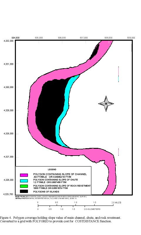
Water surface elevation and slope were estimated using two methods. When field-surveyed elevations were lacking, the theoretical Construction Reference Plain (CRP) tables developed by the U.S. Army Corps of Engineers (USACOE 1990) were used for gross estimates of water-surface elevations. The CRP is a sloping, imaginary datum, nominally at an elevation that is inundated 75 percent of the time. The CRP tables provided the elevation of the CRP for the river stage gages and for each river mile. The elevation of the river level relative to CRP was known for the time of survey, and it was assumed that the water-surface elevation at the field site was the same relative to local CRP. Hence, the stage above CRP at the gage was added to the elevation of CRP at a chosen river mile, resulting in an estimate of the elevation for the surface of the river. For a section of river, in particular the uncharted chute, slope was determined as the difference in CRP elevation divided by the distance in river miles. Slope was converted to the units of the cell size of the grid (feet/meter) and each slope class was assigned to a polygon. This polygon coverage was converted to a cost grid for use in the COSTDISTANCE function in GRID.
Thus, for the CRP method, a polygon coverage was created to hold the slope value for each area: change in elevation/grid cell unit, (feet/meter) (Fig.4 ).
Grid: cost_grd = polygrid(costpoly, slope)
> costpoly – the name of the polygon coverage that contains the item
holding the cost.
> slope – the name of the item in the coverage that holds the cost values.
The COSTDISTANCE function also requires a source grid to designate a starting location from which cost is accumulated up-river. A source point grid was created with the GRID SELECTCIRCLE command with a radius of 10 meters. The channel feature coverage was used to set the map extent and overlaid on the floodplain_grd (created from the DEM) in GRID to aid selection of the point. (See Appendix for discussion of preparation of supporting coverages).
Grid: source_grd = selectcircle (floodplain_grd, *, 10, inside)
> floodplain_grd - is the grid that the command derives the cells from. The mask grid could also have been used.
> * - activates the mouse for user to select a point on the grid or coverage.
> 10 – requests the source point occupy a radius of 10 surface units (meters).
> inside – is the keyword that designates that the cells inside the 10 meter radius will be retained and all others will have NODATA values.
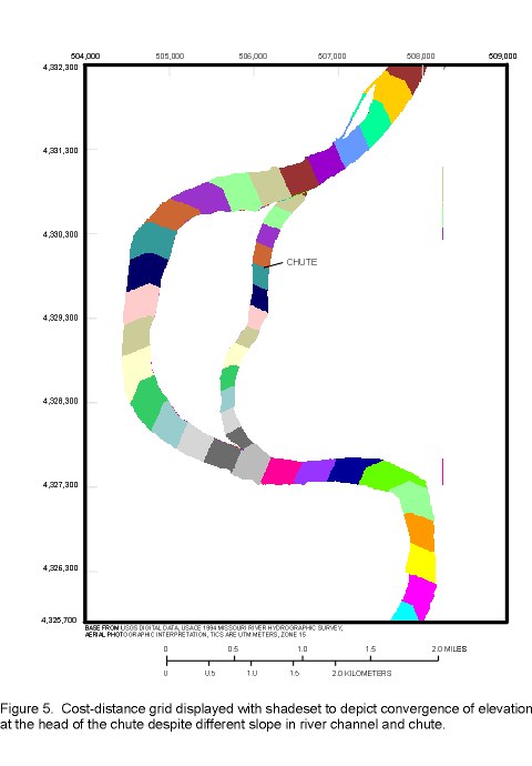
Grid: costdist_grd = COSTDISTANCE(source_grd, cost_grd)
The cost-distance grid contains an accumulation of the appropriate water-surface slope values (Fig 5 ). To make the slope meaningful topographically, it must be combined with the elevation of the source point. The surface elevation of the source point was determined and with appropriate masks set, a grid was created containing only that value. This is referred to as a value_grid in the GRID COSTDISTANCE syntax.
Grid: value_grd = 599.38
This source-point elevation grid is then added to the cost-distance grid in a separate step in order to model the water's surface in elevation units.
Grid: surface_grd = costdist_grd + value_grd
The second method seeks to improve on the first by decreasing dependence on the CRP. Because channel geometry varies substantially along the river, we know that the difference between actual water-surface elevations and CRP elevations are not the same along the river for a given discharge. Similarly, slope can be expected to vary with discharge and will not always be parallel to the CRP. To improve on the first method, two (or more) actual water-surface elevations were measured in the field on the day of data collection using conventional surveying techniques and established elevation bench marks. These water-surface elevations were then used to constrain the elevation and slope of a computed water-surface datum. In the AML, cost is first estimated as the difference in elevation between the two points and several iterations of adjustments to the slope estimate are made and tested until it provides a sufficient match of the surveyed, up-river elevation. The methods are mechanically and principally nearly the same.
Preparation of Bathymetric data:
Bathymetric data was received as a comma delimited text file with a unique record number preceding the easting, northing, and depth values. Using a simple program, the files were edited to conform to the point generate file format by changing the record number to 1 and appending END as the last line (Esri 1994). Data for each day of sampling were taken through the entire process separately.
Preparation of the Bathymetry TIN:
A TIN was created from the bathymetric points using the CREATETIN function. The map extent was reduced to the area of interest using the xmin, ymin, xmax, ymax coordinates, obtained from a coverage with the WHERE command in ARCEDIT. The generate files containing depth measurements are entered as mass points. The 9997 device allows you to view the TIN in hyposmetric shading during its creation. Weed and proximal tolerances, and densify intervals were set to 3 meters. The –1 z-factor gives the depth attribute a negative value. The z-factor can also be used to convert from feet to meters or meters to feet. For example:
Arc: Createtin <tinname> weed proximal zfactor xmin ymin xmax ymax device
(1) Arc: CREATETIN depthtin1 3 3 –1 504209.9 4325562.4 508291.4 4331536.5 9997
(2) Generate day1.txt point mass
(3) Cover bndy_poly poly elev hardclip
(4) End
Explanation of Commands:
Bathymetry grid:
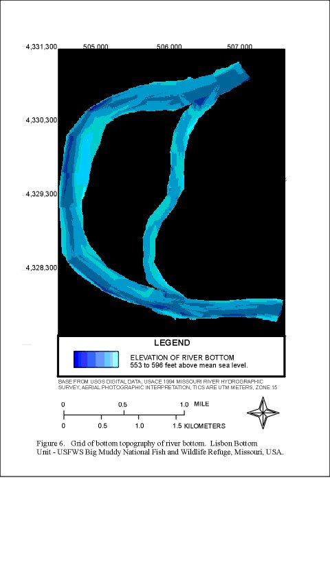
The depth TIN was converted to a lattice with the TINLATTICE command; then in GRID, with the islands and floodplain masked out, the lattice was converted to a grid. Using Map Algebra the negative depth grid was combined with the water-surface elevation grid to produce the bathymetry grid which had values in feet above mean sea level (Fig. 6 ).
Arc: TINLATTICE depth_tin1 depth_lat1 linear 1 float
Grid: depth_grd1 = depth_lat1
Grid: bath_grd1 = surfgrd1 + depth_grd1
In the second method, each day’s depth data were converted to lattices. Water-surface elevation grids were derived for each day, and the depth grid was subtracted from the grid. A condition statement was used to replace the part of the water-surface elevation grid without depth data with NODATA. The bathymetry grids are then ready to be merged.
Final Floodplain grid:
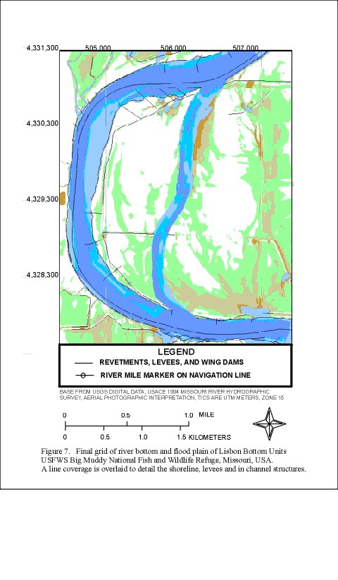
The bathymetry grid was merged with the floodplain grid derived from the DEM using the MERGE command (Fig. 7 ). The MERGE command was used instead of MOSAIC in this instance because MERGE selects one grid’s elevation value over another, giving higher priority to the grid listed first. Here, the bathymetric grid values were given preference over the floodplain values.
Grid: Final_grd = MERGE(bath_grd1, bath_grd2, floodplain_grd)
Surface TIN:
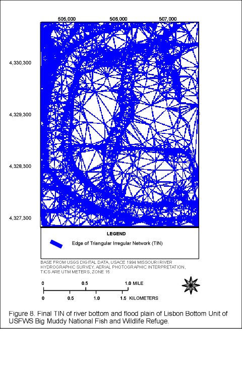
The final grid is converted to a TIN with the LATTICETIN command (Fig. 8 ).
Arc: LATTICETIN final_grd final_tin
Post processing:
Often when describing relatively flat surfaces with TINS, flat triangles result. These are not easily remedied and require substantial reprocessing (Leonard and Coughlan 1997). Once the tin is produced and evaluated, new breaklines or points may need to be added to the tin.
CONCLUSION
Surface-water hydraulic modeling is an essential tool in inventorying the temporal and spatial variation of habitats of the Missouri River. In order to more completely represent the ecology of habitats of the Missouri River, the connection between the flood plain and river must be modeled. Fish and wildlife use aquatic habitats of both the channel and the flood plain when conditions such as depth, velocity, and temperature are suitable. Identifying the range of conditions that are suitable for use by fish and wildlife over time may provide guidelines for river and flood plain management.
One of the main challenges in modeling rivers and flood plains is to handle the necessarily large quantities of data required by these models. The procedure described here has been shown to be a useful and efficient geospatial tool for integrating topographic and bathymetric data over varying discharges.
REFERENCES
DeLonay, A. J., E. E. Little, C. F. Rabeni. Personal Communication. Approaches for Monitoring Pallid Sturgeon Movement and Assessing Habitat Use in the Lower Missouri River, USA. Proceedings of the International Society on Biotelemetry.
Dugger, K. M. 1997. Foraging Ecology and Reproductive Success of Least Terns Nesting on the Lower Mississippi River. Doctoral Dissertation. University of Missouri Columbia 137 p.
Esri 1994. Understanding GIS. The ARC/INFO Method. Environmental Systems Research Institute, Inc. p.4-44-4-52.
Gordon, N.D., McMahon, T.A., Finlayson, B.L., 1992. Stream Hydrology: An Introduction for Ecologists: Wiley & Sons, Chichester, England, 526p.
Hesse, L.W., J.C. Schmulbach, J.M. Carr, K.D. Keenlyne, D.G. Unkenholz, J.W. Robinson, G.E. Mestl. 1989. Missouri River Fishery Resources in Relation to Past, Present, and Future Stresses. P 352-371. In D.P. Dodge (ed.) Proceedings of the International Large River Symposium. Can. Spec. Publ. Fish. Aquat. Sci. 106.
Leonard, T. J. and D. J. Coughlan. 1997. Reservoir Bathymetry – Mapping the Pitfalls. Esri International User’s Conference. Environmental Systems Research Institute, Inc. July 8-11, 1997. San Diego, CA, USA.
Panfil, M. S. and Jacobson, R.B. 1999. Hydraulic modeling of in-channel habitats in the Ozark Highlands of Missouri: Assessment of physical habitat sensitivity to environmental Change: online document, URL: http://www.cerc.usgs.gov/rss/rfmodel/
Tibbs, J.E. 1995. Habitat use by Small Fishes in the Lower Mississippi River Related to Foraging by Least Terns (Sterna antillarum). M.S. Thesis. University of Missouri, Columbia, Missouri, USA. 149 p.
Tibbs, J.E. 1997. Larval, Juvenile, and Adult Small Fish Use of Scour Basins Connected to the Lower Missouri River. University of Missouri. Final Report to Missouri Department of Conservation. 133 p.
USFWS. Ecological Services. North Kansas City MO. 1980. Missouri River Stabilization and Navigation Project, Sioux City, IA to Mouth. Detailed Fish and Wildlife Coordination Act Report. Kansas City Districts. US Army Corps of Engineers. 77p.
U.S. Army Corps of Engineers Kansas City District. 1990. Missouri River, Rulo Nebraska to the Mouth. 1990 Construction Reference Plane. River and Lake Engineering Section Hydrologic Engineering Branch Engineering Division. 31p.
Waddle, T., Bovee, K., Bowen, Z., 1997. Two-dimensional habitat modeling in the Yellowstone / Upper Missouri River System: North American Lake Management Society (NALMS) meeting in Houston, TX (December 2-4 1997, online document, URL:http://smig.usgs.gov/SMIG/features 0398/habitat.html.)
Appendix A
Preparation of supporting coverages and grids: island masks, cost polygons:
A reference coverage for this project included channel features such as the river shoreline, river mile markers, and rock revetments. The shoreline of the chute that formed only recently, was mapped by traversing the shoreline 1 meter from the water’s edge with a GPS unit; GPS data were differentially corrected to sub-meter accuracy. The shoreline coverage was then buffered by 1 meter and generalized so that vertices were 20 meters apart before it was combined with the rest of the channel polygon coverage. Water level at the time the shoreline coverage was collected was reasonably close to the water level when the bathymetric data were collected. This coverage was used to create masks and to provide outlines for the cost polygon coverage.
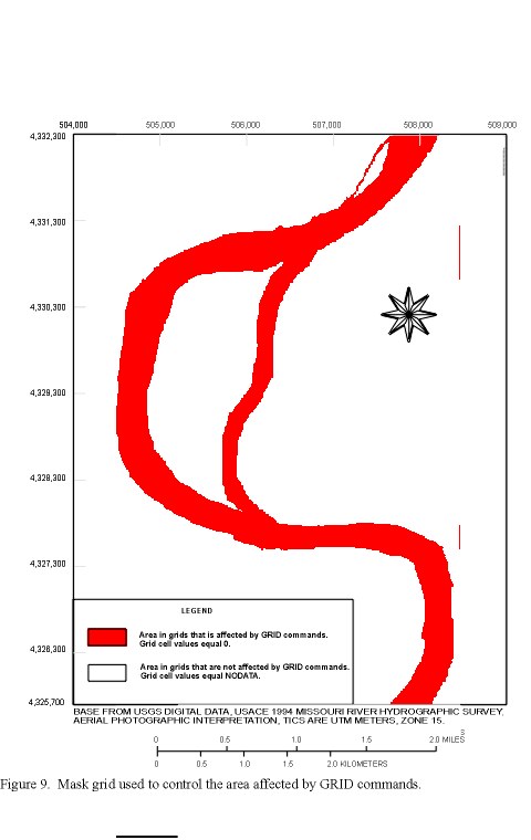
Masks of the islands and flood plain were created using the GRID SELECTPOLYGON command using the INSIDE/OUTSIDE options.
Grid: Island-mask = selectpolygon(floodplain_grd, island_poly, outside)
> Floodplain_grd – the grid from the DEM is used to provide the cells
for the command.
> Island_poly – a polygon coverage of only the islands
> Outside – keyword that sets the cells inside to NODATA and the cells
outsided the polygon to 0.
To complete the final mask, the island mask is set, and the SELECTPOLYGON command is issued with a polygon of the river’s outer shore and with the "inside" keyword (Fig. 9 ).
Ellen Ehrhardt, Biologist, USGS-BRD Columbia Environmental Research Center, 4200 New Haven Road, Columbia, MO 65201.
Robert B. Jacobson , Geomorphologist, USGS-BRD, Columbia Environmental Research Center, 4200 New Haven Road, Columbia, MO 65201,Robb_Jacobson@usgs.gov
Aaron J. DeLonay, Ecologist, USGS-BRD Columbia Environmental Research Center, 4200 New Haven Road, Columbia, MO 65201, Aaron_Delonay@usgs.gov