M. De Maio
Italian National Research Council (GNDCI – CNR), C.so Duca degli Abruzzi 10128 Torino; E-mail: mdemaio@athena.polito.it

1. INTRODUCTION

Italy as a whole has adequate groundwater resources which supply the main source of drinking water. A forecast of the 2000s would indicate a total demand of 100 Gm³/y for human, industrial and agricultural uses compared to a total availability of 200 Gm³/y. Stretching through more then 10 degrees of latitude between the Alps mountain chain and Africa, the climate in Italy ranges between a semi-arid type, in the southern areas, to sub-humid and humid conditions in the northern perimountain and mountain region. The atmosphere dynamics give severe drought periods in some locations and, in the late summer and autumn, the frequent occurrence of a sort of very concentrated and violent tropical storm that causes flash floods which are very difficult to forecast. The impact of this type of flood is frequently a severe disaster that strikes the communities by destroying housing and activities, motorways, aqueducts and pipelines, animal husbandries, stockpiles, and all the pollution preventers, such as waste disposals, sewerage, cesspools and septic tanks, wastewater treatment plants, etc. The high rate of contaminants discharged into the soil and water environment causes a generalised contamination hazard for surficial and groundwater resources throughout the flooded area. The situation of the involved communities becomes worse during the post-event, due to a water supply crisis that occurs because of the destruction of the wells, spring tapping and the adduction network, as was surveyed in the Tanaro river basin (about 6000 km² in the north-west of Italy) which was severely impacted by a flash flood in November 1994.

The groundwater contamination hazard can be judged to be more or less high according to the degree of intrinsic vulnerability of the subjected aquifer, i.e. the specific susceptibility of an aquifer system to ingest and diffuse hydro-vectored contaminants whose impact on the groundwater quality is a function of space and time. The assessment of the intrinsic vulnerability has to be performed through a classic zoning technique via GIS, using a great deal of available parameters that are elaborated by a count point system model (Civita, 1994; Vrba & Zaporozec, 1995). The outputs that are supplied to decision makers consist of a groundwater vulnerability integrated map of the single involved Municipality territory and the option of performing dynamic scenarios of any area in the investigated zone to enforce proper actions in order to prevent the contamination impact.

In this paper, one of 74 investigated Municipality areas is presented as a case history to illustrate the used approach and the obtained results.

2. CASE HISTORY

The territory of the Municipality of Quattordio (» 18 km²) is located in the central part of the main course of the Tanaro river, between Asti and Alessandria, the towns most damaged by the 1994 flood event. The area is gently hilly going southward towards the flood plain. The hilly area is crossed by two normally dry streams, that may be subject to instantaneous floods in rainy periods. The hilly zone is vine cultivated, while in the plain traditional and specialised agriculture prevail.

The hydrogeological structure of the area is characterised by a basal sandy complex (Asti Sand) on which a relatively thick alluvium deposit that is typical of a broad flood plain, can be found (alternations of sand and clay layers going upward to coarse grained recent sediments). Within these deposits, a water table aquifer that is discontinuously semiconfined in some places, can be found. The recharge of the aquifer is due to the close linkage to the surficial network and locally is largely developed by a number of wells. The flash flood of early November 1994 inundated the whole flood plain leaving, when the flood water receded, a mud cover containing a great deal of pollutants (hydrocarbon, heavy metals, sewerage sludge, animal waste carcasses and so on) of urban, industrial and agriculture-breeding origins.

On the basis of available data, an aquifer vulnerability assessment was soon performed and an integrated vulnerability map was constructed using the point count system model sintacs, properly structured to be implemented by ArcInfo GIS. sintacs (Civita, 1990; 1993; 1994; Civita & De Maio, 1997), originally shaped in a similar way to drastic (Aller et al. 1987), has become different, since 1990, together with the Italian CNR funded research advancement and a great deal of tests which were carried out for the first three releases. Release 4 which was used for the assessment of the aquifer vulnerability of the flooded zone, retains only a small part of the very effective drastic skeleton. It is a true evolution of the preceding three releases, particularly because of the automation carried out by means of the hardware and software of very wide diffusion and usage. The model is based on the following parameters that were previously transformed into the 1 to 10 rating range:

• depth-to-water table, that is, the depth of the piezometric level (both for confined or unconfined aquifers) in comparison to the ground surface;
• effective infiltration action which is very significant because of the dragging down surface of pollutants and, on the other hand, their dilution, at first during the travelling through the unsaturated zone and after within the saturated zone;
• soil/overburden attenuation capacity, the first defence line of the hydrogeologic system where several important processes take place inside the soil which makes up the attenuation capacity;
• unsaturated zone attenuation capacity, i.e. the second defence line of the hydrogeologic system against fluid or hydrovectored contaminants;
• hydrogeologic characteristics of the aquifer, i.e. the process that takes place below the piezometric level when a contaminant becomes mixed with groundwater after having lost a small or more relevant part of its original concentration while travelling through the soil and unsaturated thickness;
• hydraulic conductivity range of the aquifer which represents the groundwater mobility capacity inside a saturated media, thus the mobility potential of a hydrovectored contaminant which has a density and viscosity that is almost the same as the groundwater;
• hydrologic role of the topographic slope which rules the amount of surface runoff produced, the precipitation rate and displacement velocity of the water (or a fluid and/or hydrovectorable contaminant) over an equal surface.

The grid square cell structure of the sintacs input data has been designed in order to use several weight strings (multipliers) both in serial and in parallel. The weight strings have been prepared to emphasise, to a lower or greater extent, the single parameter’s rating in order to satisfactorily describe the effective hydrogeologic and impacting situation as it is set up by the sum of data. The present release of sintacs presents 5 weight strings (normal impact, relevant impact, drainage from surficial network, deep karstified terrain and fissured terrain). The percentized product of the ratings for the weights gives the vulnerability index which is shaped into 6 vulnerability degrees to make the map. The work is completed by overlaying the flow net, the census of the contamination spreading centres (CSC) and the hazard targets (wells and springs) on the intrinsic vulnerability map that thus become a very strong planning tool even for the post-event of a natural disaster.

3. ArcInfo IMPLEMENTATION

Grid of Depth-to-water

The depth to water map was obtained in an automatic manner through subtraction between the grid of the height of the topographic surface and the grid of the piezometric surface heights. The topographic surface was obtained using the Piedmont Region DEM (Digital Elevation Model). DEM is not compatible with ArcInfo and this fact determined the necessity of preparing opportune software in DOS in order to transfer the original files to an ASCII file that is compatible with ArcInfo. The x, y and z coordinates were used as the points that make up the DEM. The obtained file was imported and suitably elaborated in order to obtain an iso-elevation area covering (1m interval) to which a 50 m side mesh has been applied (GRID1). The isopiezometric map (?h = 1m) was produced from the surveyed data by linear interpolation using a traditional method, digitized with ArcInfo. The production of the topology has permitted the attribution of the mean elevation of the isopiezometric level to the isovalue area (GRID2).

The fact that DEM was made compatible to the ArcInfo ambient is, in itself, an extremely important result. DEM is accurately precise and the extraordinary potentiality of GIS makes it usable in many land applications (planning of infrastructures of mean scale denomination, study of landslide phenomena, etc). Furthermore, in this context, the obtained elaboration constitutes a great innovation of the traditional techniques for the compiling of depth to water maps. These, even in situations of slight variability of the topographic surface, do not finish noteworthy accuracy and, above cell, the automatic elaboration makes them available almost in real time (Fig. 1).

Figure 1 - Flow chart of Depth-to-water Map

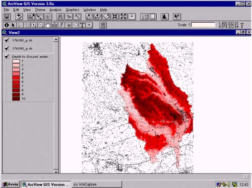
The depth-to-water grid was then reclassified in the intervals for seen by the sintacs method (Fig. 2).

Figure 2 – Depth-to-water Grid

Grid of effective infiltration action

The infiltration map was obtained through the construction of an effective infiltration value map of the studied areas from the yearly average rainfall and average temperature data compared, cell by cell, to average elevation. The effective average evapotranspiration was calculated by Turc expression for only some areas within which the soil cover is thin or absent, whilst for the others the expressions for thick soil were used which do not need the evapotranspiration value (Civita, 1994). The potential infiltration coefficient for thick soils (?) was determined on the basis of the soil type by means of the abacus given by the sintacs methodology (Civita & De Maio, 1997).

The thus obtained elaborated map was digitized in ArcInfo, the topology was constructed and the infiltration values were assigned to the various areas. The usual mesh was applied to this coverage (Fig. 3).

Figure 3 – Effective Infiltration Grid

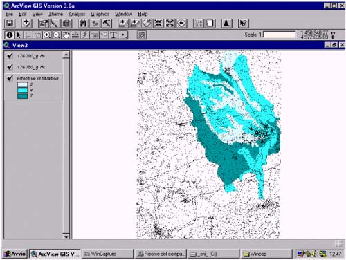
The thus obtained grid was then reclassified for the assignation of the sintacs points relative to the infiltration intervals shown in the same method (Fig. 4).

Figure 4 - Flow chart of effective infiltration map.

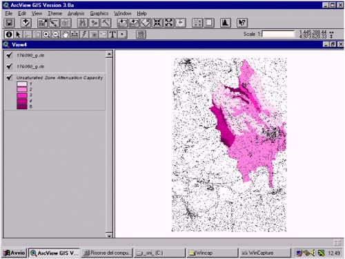
Grid of Unsaturated zone attenuation capacity

The map relative to the autodepuration effect of the saturated zone was obtained through mapping and successive digitizing. The ratings forseen by the sintacs method were attributed to homogeneous areas on the basis of the lithological conditions of the unsaturated zone thickness. The topology was build and the related points were attributed to each areas. The usual mesh was applied and the grid of the sintacs ratings for the unsaturated zone was thus obtained (Fig. 5). The used procedures are the same that were carried out for the infiltration map and therefore not shown of the flow chart.

Figure 5 – Unsaturated Zone Attenuation Capacity Grid

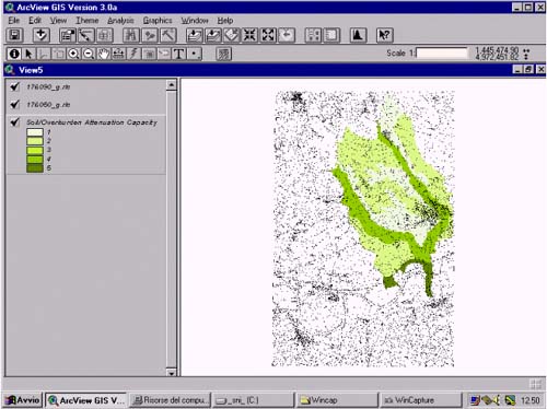
Grid of soil/overburden attenuation capacity

The type of covering map was taken from the study on the soil capability (IPLA, 1982) and from available pedology data (1991-1995 samplings groups). The mapping was carried out using traditional methods and the obtained elaboration was digitized into ArcInfo. The topology was created and the relative ratings were assigned according to the reference abacus of the sintacs method. The usual mesh was applied and the grid for the covering type was obtained with sintacs ratings (Fig. 6).

The followed procedure is the same used for the production of the infiltration grid, without the reclassification which was not necessary.

Figure 6 – Soil/Overburden Attenuation Capacity Map

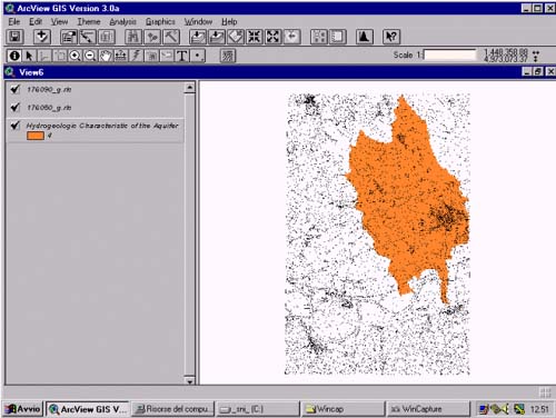
Grid of hydrogeologic characteristics of the aquifer

The map of the hydrogeologic characteristics of the aquifer was obtained by attributing sintacs ratings according to the abacus given in the same method.

The same ratings were attributed to the whole area as the studied aquifer was always the same. The usual grid was applied to the thus obtained coverage (Fig. 7) by a very simple procedure.

Figure 7 – Hydrogeologic Characteristics of the Aquifer

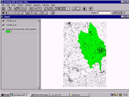
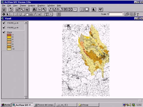
Grid of hydraulic conductivity

The hydraulic conductivity map was obtained for each studied area by means of the attribution of K values that were determined by means of recovery tests. The procedures for the production of the coverage of this parameter and of the sintacs rating grid (Fig. 8) was the same as that used for the infiltration grid (digitizing, building topology, application of the mesh and reclassification).

Grid of Slope

The slope grid was obtained in a completely automatic manner. The potentiality of ArcInfo is such that it allows one to use a command that creates polygonal slope coverage (SLOPE) for the origination of the LATTICE (three-dimensional grid derived from TIN). This coverage is defined through the indication of an opportune file during the elaboration of the stage of the slope interval percentage that one wants to map. The sintacs method indicates the slope intervals and the points assigned to these intervals.

Figure 8 – Hydraulic Conductivity of the Aquifer Grid

Figure 9 - Flow chart of the slope map

The mesh of the slope coverage was however applied (Fig. 9). The obtained grid was reclassified for the assignation of the relative sintacs ratings (Fig 10). The importing of DEM into ArcInfo by the Piedmont Region is described in the procedure used for the depth to water map.

Figure 10 – The Slope grid

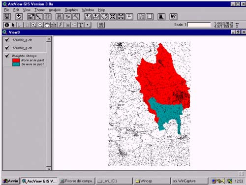
Grid of weight strings

Only two (Normal impact and Severe impact) of the five situations forseen by the sintacs method exist in the studied area. The map and the relative grid were constructed using the standard procedure: traditional mapping, digitizing, topology production and application of the usual mesh (Fig. 11).

Vulnerability Map

The vulnerability map was obtained through the implementation of a cell by cell procedure, in the GRID ambient, in AML which forsees:

1. Verification of the cells in the hydrogeologic impact characteristics grid and location of the relative weight line.
2. Application of

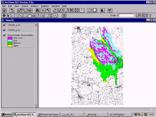
The value of the sintacs index of the single cells was then normalized through the implementation of a further cell by cell application procedure. One of the 6 intervals of the index value, identified by the sintacs model, was assigned to each cell which was completed with a colour code ranging from red (extremely high Vulnerability) to violet (extremely low Vulnerability).

The normalized intrinsic vulnerability grid was thus obtained. The whole CSC, the average ground water flow net and the whole contamination hazard targets (springs, wells and related protection areas systems) were then added to the grid thus obtaining the Integrated Vulnerability Map (Fig. 12).

Figure 11 – The Weight Strings Grid

Figure 12 - The Groundwater Vulnerability Grid

4. FINAL REMARKS

The illustrated approach is now in progress to be completed for each of 74 Municipality impacted by the 1994 flash flood in the Tanaro valley. It will therefore possible to use the integrated vulnerability map to forecast the areas under groundwater contamination hazard and the effects of a possible new flood (the calculated return period is almost 20 years) will be minimised by a new disaster planning. All the implemented information will be used, also, within the master plan and the single Municipality planning scheme to re-locate the main withdrawal points and a lot of CSC and activity impacted by the flood.

References

• Aller L, Bennet T., Lehr J.H., Petty R.J., Hackett G. (1987) - DRASTIC: A standardized system for evaluating ground water pollution potential using hydrogeologic settings. NWWA/EPA Ser., EPA600/287035. 455 p., 11 Maps (with included references)
• Civita M. (1987) - La previsione e la prevenzione del rischio d'inquinamento delle acque sotterranee a livello regionale mediante le Carte di Vulnerabilità.. Proc. Cong. "Inquinamento delle Acque Sotterranee: Previsione e Prevenzione", Mantova.
• Civita M. (1990.a) - La valutazione della vulnerabilità degli acquiferi. Proc. 1° Nat. Cong. "Protezione e Gestione delle Acque Sotterranee: Metodologie, Tecnologie e Obiettivi", 3, Marano sul Panaro,.
• Civita M. (1990) - Legenda unificata per le Carte della vulnerabilità dei corpi idrici sotterranei/ Unified legend for the aquifer pollution vulnerability Maps. Studi sulla Vulnerabilità degli Acquiferi, 1 (Append.), Pitagora Edit. Bologna. 13 p.
• Civita M. (1993) - Ground Water Vulnerability Maps: A Review. Proc. IX Symp. Pesticide Chemistry "Mobility and Degradation of Xenobiotics", Piacenza , p. 587-631.
• Civita M. (1994) - Le Carte della vulnerabilità degli acquiferi all'inquinamento: Teoria & Pratica. Pitagora Editrice, Bologna, 325 p.
• Civita M. (1995) - Sul rischio di inquinamento delle risorse idriche sotterranee. Proc. 2° Nat. Cong. "Protezione e Gestione delle Acque Sotterranee: Metodologie, Tecnologie e Obiettivi", Nonantola (Modena), 4, pp. 103-119.
• Civita M., De Maio M. (1995) - L’analisi per scenari dinamici di situazioni ambientali a rischio multiplo di degrado delle acque destinate a scopi potabili. Bull. GEAM 32, 4 (1995), p. 233-238.
• Civita M., De Maio M. (1997) - SINTACS. Un sistema parametrico per la valutazione e la cartografia della vulnerabilità degli acquiferi all’inquinamento. Metodologia & Automatizzazione. Vol. 60 - Pitagora Editrice, Bologna.
• IPLA (1982) - Capacità di uso dei suoli.
• Vrba J., Zaporozec A. (Editors) (1994) - Guidebook on Mapping Groundwater Vulnerability, Intern. Cont. to Hydrogeol., 16, 131 p. - Heise Ver. Edit. Hannover (1995).