Title
Author’s Name
Abstract
Paper Body
References
Acknowledgements
Author Information

Jeffrey B. Miller

Using GRID for Regional Population,

Agriculture and Natural Hazards Modeling

Abstract

Population increase and migration into areas under threat of natural hazards is a global concern. Earthquakes, tsunamis, volcanoes, cyclonic storms and floods endanger increasing populations and their sustaining agriculture.

Earth Satellite Corporation worked with iSciences, L.L.C. to develop a GIS that synthesizes the relationship of regional population increase, the value of sustaining agriculture and natural hazards (earthquakes, tsunamis, volcanoes and cyclonic storms) that threaten them. The GIS includes ArcInfo scripted models, map databases, statistics, cartographic products and ArcView projects for the Tigris-Euphrates (including Iraq, Syria and Turkey), Indonesia, Nigeria, and South Asia (including India, Pakistan, and Bangladesh) regions.

to index

Using GRID for Regional Population,

Agriculture and Natural Hazards Modeling

Critical Questions

Earth Satellite Corporation teamed with iSciences to address three critical geographical questions. Firstly, what is the location and extent of population and agriculturally prime areas at a regional scale? Secondly, what is the location and extent of natural hazards such as earthquakes, floods, cyclonic storms, desertification, tsunamis and volcanoes? Lastly, what is the relationship between population, agriculture, and infrastructure with natural hazards? Using raster-based GIS modeling these questions could be addressed.

to index

Study Area

The project selected a number of geographically diverse study areas for regional-scale analysis. South Asia, including Bangladesh, India, and Pakistan, the Tigris Euphrates region, including Turkey, Iraq and Syria, in addition to Nigeria, and Indonesia were chosen for analysis. The analysis was conducted at 1 km² cell resolution.  

to index

Data Sources  

Publicly available data and information served as the source of inputs to the GIS analysis.

Attribute population information was collected from a number of sources. Typically, national level population information in the form of local national censuses was obtained from the International Division of the US Bureau of Census. National level population information was readily available on the US Bureau of Census International Division web site.

Vector-based spatial data was likewise obtained from publicly available sources. Spatial data contained in the Defense Mapping Agency’s 1:1,000,000 Digital Chart of the World (DCW) served as a complete source of regional-scale base information.

Raster structure spatial data were also acquired from publicly available sources. NOAA provided a number of data sets including precipitation and desertification hazard. The International Geosphere Biosphere (IGBP) program provided global 1 km² land cover. The NOAA DMSP program provided global coverage of nighttime persistent bright lights. The USGS EROS data center’s GTOPO30 database served as an elevation model.  

to index

Hardware and Software

Earth Satellite Corporation’s Sun Enterprise 4000 and StorageTek 9710 Library Storage Module was the primary hardware resource for the project. Analysts also used Intel Xeon personal computers for client connectivity and analysis work. Operating system software included SUN Solaris and Windows NT 4 (SP 6). GIS software included Environmental Systems Research Institute’s ArcInfo 8. All analytical processing was conducted using ArcInof GRID. Cartography was conducted using ArcView 3.2. Some image processing was conducted using ERDAS Imagine 8.3.  

to index

Findings and Methods

The project developed a series of models to address the critical geographic questions identified. These included population density, agricultural primeness and natural hazards models. The resulting output surfaces were combined to identify population, agriculture and infrastructure exposed to significant natural hazards.

Population Models

The project produced km² resolution population density for the late 1990s and forecasted 2010 population. The model is a disaggregation of first order administrative (state/provincial) population to the km² level.

to index

Rural Population

State-level rural population totals for all countries were obtained through the US Department of Commerce US Census Bureau International Program. These state-level rural figures were allocated to 1 km² pixels based on a multicriteria suitability model.

A surface of total suitability based on multiple criteria was developed for rural areas. Higher suitability areas would receive higher proportions of the total state level population. Criteria for rural population allocation included

Urban Population

Urban population density modeling took a similar approach. State level urban population estimates from local national censuses were allocated to the cellular (1 km²) level. A different criteria set was applied in the allocation:  

US Census Bureau estimates of national level population for each country for 2010 were available online. The subnational urban and rural population estimates available from local national censuses were proportionally weighted to produce 2010 state level population estimates. These estimates were then used as inputs through the same allocation process described above for km²-level population modeling.

The resulting urban and rural population density GRID surfaces were combined to produce a complete population density per km² surface for 1998-9 and 2010 for all study areas.

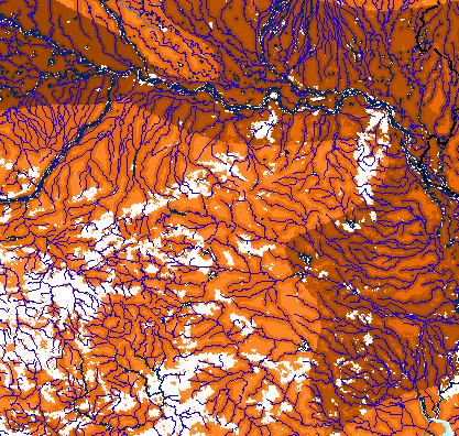
Population Density 1998, India-Bangladesh Boundary Region. Gray areas denote lowest density regions, while higher population densities are portrayed in yellows, oranges and reds.

to index

Agricultural Primeness

The project developed a surface of agricultural primeness, or suitability of the landscape for agricultural use. The model used two compound weighted criteria (physical and socio-economic factors) to index suitability in a raster surface:

1. Physical Characteristics

These layers are modeled to reflect the physical characteristics of the landscape that favor agriculture. The three selected component criteria were soils, moisture availability and land cover:  

2. Socio-economic Characteristics

A single socio-economic layer that reflects access to demand centers for agricultural products was produced. This surface assigns high agricultural primeness scores to areas that have easy access to higher density population centers, and lower agricultural primeness scores to areas that have poor access to low-density population centers:  

The result is a composite agricultural primeness GRID surface that shows relative suitability of the landscape for agriculture.

Primeness of Agricultural Lands, India-Bangladesh Region. Lighter browns indiciate more marginal, lower-suitability for agriculture. Darker browns indicate areas with high primeness for agriculture.

to index

Natural Hazards

A series of natural hazards surfaces were modeled and compiled from existing sources.

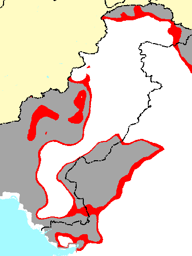
Earthquake

The earthquake hazard surface portrays the likely damage in Mercalli scale over the next fifty years from Earthquakes. Earthquake data was obtained from ‘The World Map of Natural Hazards’, Munchener Ruckversicherungs-Gesellschaft, as provided by the UNEP GRID Natural Hazards Database on Earthquakes and ingested to the GIS.

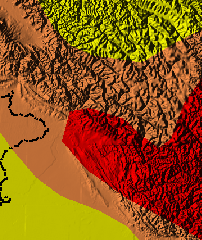
Earthquake Hazard, India-Pakistan Boundary Region. Yellows indicate lowest earthquake hazard, while oranges and reds indicate highest potential damage from earthquakes.

to index

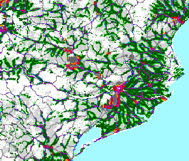
Topographic Flood Hazard

The flood hazard model assesses the topographic risk of flooding throughout the project study areas. The flood hazard map is not event specific. Instead, the model assesses all areas for the relative cost of water migration from a source inundated area or river to derive flooding potential. Flat areas close to rivers, and areas near wetlands are characterized as more subject to flooding. A topographic cost surface that models the cost of migration of water from source wetlands and rivers is produced and interpreted to identify risk of flooding. Areas of lower cost of water migration are assigned higher risk values, while areas of higher cost of water migration are given lower risk values.

Source rivers, streams and wetlands were obtained from the 1:1,000,000 Digital Chart of the World (DCW). Source elevation data was obtained from the EROS data center 1996 30 Arc Second USGS gtopo30 map database.  

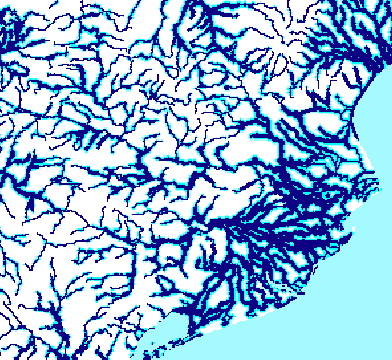
Topographic Flood Hazard, Orissa Region, India. Light blues indicate lower flood potential, while darkest blues show areas of greatest hazard.

to index

Cyclonic Storms Hazard

The storm risk model maps the regional historical density of cyclonic storm intensity from November 1971 to November 1995.

All historical cyclonic storm and tropical depression center tracks recorded from 1971 – 1999, provided by NOAA historic data compiled by Global Tracks, served as model input.

The regional line density (within a 500 km distance) of cyclonic storm and tropical depression center tracks was calculated for each 1 km² cell in the study area. Storm intensity was used as a weighting factor in modeling regional density. Tropical depressions represented the lowest line density weight, and higher category typhoons/hurricanes were given higher line density weightings. The resulting weighted density surface was then categorized into low, low-moderate, high-moderate, and high-risk categories to represent risk variance.

The result is a risk surface GRID showing the historical (1971 - 1995) risk of cyclonic storms and tropical depressions throughout the study areas. The risk surface represents the regional frequency, density, and intensity of cyclonic storm activity.

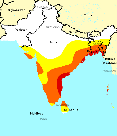
South Asia Cyclonic Storm Hazard. Lowest hazard is shown in yellow, while greatest historical storm density areas are portrayed in red.

to index

Desertification Hazard

The desertification layer actually expresses the deserts of the study area as well as a rim of potential desertification. The layer used in this study is derived from a dataset created by David Hastings of NOAA (Hastings and Di 1993).

The original layer was based on NOAA AVHRR imagery. The imagery was processed earlier as part of NOAA's Global Change Database (GCDB), which consists of NDVI processed AVHRR imagery. It is a collection of monthly global NDVI compilations produced from April 1985 to December 1988 and derived from NOAA’s Global Vegetation Index (GVI) (Hastings and Di 1992). The GVI was created by producing weekly NDVIs of AVHRR data and then removing the highest and lowest values of each image, then taking the root mean square of the remaining values. Then this information was composited into monthly data. This was done to reduce spurious NDVI high values and some cloud contamination (Hastings and Di 1992). This data was analyzed to determine areas of no vegetation growth. The number of years the data covers and the many months of data utilized negated the effects of short-term drought causing an over-estimation of desert area, or the under-estimation of desert due to rare precipitation (Hastings and Di 1992).

Next a “fragile fringe” or marginal zone between desert and vegetated areas was determined using NDVI analysis as well. Also, local expertise was used in North Africa and the Arabian Peninsula to detect the threshold between these land cover types. Values below 56 on an 8-bit image were labeled as desert. The fringe areas were placed at 57-76. These fringe areas include irrigated desert areas used for agriculture. The marginal areas are interpreted as sparse vegetation on the edges or within deserts that are at risk for desertification. Some areas expressed as marginal are surrounded by healthier vegetation. Hastings interprets these areas as damaged by overgrazing or other wasteful activities (Hastings and Di 1992). Values over 76 are expressed as vegetated areas. This methodology has produced the most accurate global map of deserts and marginal areas (Hastings and Di 1992).

This data set is unavailable to the public due to its having been misplaced by its principal investigator. Therefore unconventional means were utilized to process this information. The web page containing the above describe data in a graphic was displayed and the gif image was saved to a local hard-drive. There it was converted to a bitmap image using Microsoft Paint, then it was converted from bitmap to tiff format using Imaging for Windows NT. The tiff file was finally imported into Imagine as a 256 class thematic layer rather than a continuous image. This was to avoid having to classify the image later, as the features were already very well separated by color. Before rectification the file was windowed to the area of study so as to minimize number of pixels to be processed and improve spatial accuracy.

In Imagine the file was rectified to the IGBP data set previously collected for this study. The original projection information was not known. The IGBP layer is also based on AVHRR imagery so it was hoped there would be some inherent similarities in the data spatially. Therefore a polynomial order of 2 was used. Eleven GCPs were used which were located around apparent water bodies. The image was resampled during the process to 1 km and a bilinear convolution resampling method was used, while the grid sampling x and y values were set at 200. After rectification, it was necessary to recode the areas around water bodies within screen-digitized AOIs because the shore values were affected by being averaged during the bilinear resampling. Then these recoded areas were mosaicked over the layer to correct this problem. The threshold for setting pixels on the shore area to water or vegetated was 56, the same as was used in the original layer to distinguish between desert and prone areas. The resulting mosaic was then subset so that its shape would be rectangular instead of the warped look inherent from the rectification. Unfortunately there is some missing data in the study area that was simply not available on the web image. All the missing area is fully vegetated however.

Since the data was imported as a thematic layer, it was readily processed into a thematic map by recoding the 256 classes into 2 and 4 classes. The 2 class map includes a desert class and an at risk class. The 4-class map includes: water, vegetated, desert, at risk. The results were exported to GRID for use in ArcInfo.

Desertification Hazard, India-Pakistan Boundary Region. Existing deserts are shown in gray, while areas prone to desertification are shown in red.

to index

Tsunami Hazard

A surface showing the potential hazard of tsunami landfall was developed from the NOAA National Geophysical Data Center Tsunami Event Database. This event database included the longitude and latitude for the epicenter of earthquakes that caused "definite tsunamis" from 1600 - 1999.

Risk was determined by modeling the cost of water movement through a friction surface based on land elevation and distance from all source tsunami earthquakes. The result was an accumulation of risk based on cost distance. Lower cost areas are typically in low-lying shore areas, closer to multiple known tsunami earthquake epicenters.

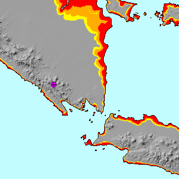
Tsunami Hazard, Jawa Barat-Sumatra, Indonesia Region. Lowest tsunami hazard areas are portrayed in yellow, while the greatest hazard areas appear in red. Known tsunami source earthquakes are shown as purple circles with crosshairs.

to index

Volcano Hazard

The Volcanic Hazard surfaces show the potential threat of volcanic activity based on Smithsonian (provided by the National Geophysical Data Center) average recorded Volcanic Eruptivity Index (VEI) for each volcano recorded. Blast hazard, and volcanic ash fallout hazard are the two component criteria applied in the model.

Blast Hazard

Blast hazard is modeled as an area at immediate risk of exposure to ejected debris and the explosive force of a volcanic eruption. The extent of this risk zone is tied to the average Volcanic Eruptivity Index (VEI) for a given volcano. Higher VEI average volcanoes have larger, more forceful explosions which pose hazard to larger geographic extents. Conversely, volcanoes with lower VEI averages have weaker explosions whose blast zones do not extend to great distances. Areas that are directly visible from a volcano caldera are potentially vulnerable to blast. Areas hidden by topography are not visible to the caldera, and are at lower risk of blast damage. The greater the VEI, the greater the distance to which blast vulnerability is modeled. Areas within this modeled blast zone receive a high risk score.

Volcanic Ash Fallout

Volcanic ash fallout hazard identifies areas that are potentially at risk of exposure to falling volcanic ash in the event of volcanic eruption. The extent of volcanic ash fallout is directly related to the average Volcanic Eruptivity Index (VEI) value for the candidate volcano. Higher VEI averages have higher plume heights and ejecta volume, and consequently fallout zones of greater geographic extent. Lower average VEI volcanoes have lower plume heights and ejecta volume. Consequently, the corresponding fallout risk zones have a more limited geographic extent. Fallout areas closer to the volcano caldera receive a higher risk score. This score decays as distance from the caldera increases.

Blast hazard and volcanic ash fallout hazard scores are combined in additive overlay to produce a risk surface for an individual volcano. The risk surfaces for each volcano in the study area are then combined into a single layer of aggregate risk. Areas that are proximate to multiple high VEI average volcanoes are at greater risk than areas that are remote to low VEI average volcanoes.

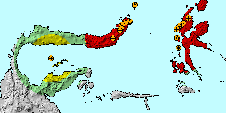
Volcano Hazard, Sulawesi Utara – Maluku, Indonesia Region. Lower hazard areas are shown in green tones, while greatest hazard areas are shown in reds. Known historically active volcanoes are shown as orange circles with crosshairs.

The series of natural hazards GRIDS directly addressed our first critical question by identifying the location and extent of the population, agriculture and the most significant natural hazards throughout our study areas.

to index

Population, Agriculture, Infrastructure and Natural Hazards

The second critical question our project proposed to answer, the relationship between population, agriculture, and natural hazards, is also addressed through GIS modeling.

Simple GIS overlay of high population density areas, transportation network information, and agricultural areas with any combination of natural hazard GRIDs will produce complex composite surfaces which show populations, agriculture and transportation infrastructure at risk.  

Population, Infrastructure and Agriculture under Flood Hazard Orissa Region, India. Areas in red are high population density areas at high risk of flooding. Areas in dark green are agricultural areas at high risk of flooding. Dark blue linear patterns are transportation infrastructure at high risk of flooding.

The total population and acreage of agricultural lands at risk may be quantified by any geographic enumeration. For instance, the following table summarizes Indian populations 1960, 1998, and 2010 by earthquake risk zone :

to index

Recommendations for Further Work

Currently the models produced do not reflect calibration based on detailed empirical data obtained from fieldwork. Many of the geographic themes produced have never been field surveyed in detail. It is anticipated that as field survey information is developed, the models will be refined and calibrated to fit the evidence contained in sources of higher accuracy.

to index

References

Hastings, David A. and Di, Liping. Characterizing the Global Environment: An Example Using AVHRR to Assess Deserts, and Areas at Risk of Desertification. NOAA NGDC, published on website: www.ngdc.noaa.gov/seg/globsys/gisdes.shtml. 1993. 10pp.

to index

Acknowledgments

The author wishes to acknowledge the contributions of David Cunningham of Earth Satellite Corporation and Douglas Way of iSciences for their direction and leadership in this GIS project. Thanks also to François Smith and Yasmine Naficy of Earth Satellite Corporation for their efforts in the project.

to index

Author Information

Jeffrey B. Miller
Staff Scientist
Earth Satellite Corporation
6011 Executive Boulevard Suite 400,
Rockville, MD 20852-3804
(301) 231-0660
FAX (301) 231-5020
jmiller@earthsat.com
http://www.earthsat.com

to index