GIS Applications in Climate and Meteorology

Recent efforts using Commercial-Off-The-Shelf (COTS) Geographic Information Systems (GIS) for applications in climate and meteorology include traditional GIS strategies for hydromet database analysis and management, and the fusion of hydromet data with traditional GIS applications. But new techniques are emerging which exploit COTS GIS features and capabilities to support the analysis of hydromet data in the GIS operating environment.

Many of today's hydromet Interactive Information Processing Systems (IIPS) are data viewers, providing limited data analysis capabilities, usually in the form of "canned" menus for common analysis functions. One IIPS operating paradigm rapidly merges data from established and trusted sources to support the "forecaster in the loop", who makes the call - a form of office automation. The GIS paradigm provides a richer analysis environment, with flexible general-purpose topological and algebraic functions supporting analysis "on-the-fly". This generality is usually achieved at high spatial resolution, but with a related sacrifice in processing speed. In addition, meteorologists find the GIS operating model to be "different and strange" enough to require a lot of retraining (many personal communications). After all, "GIS was developed only recently to map cartographic data which change on geologic time scales, right?" Wrong - GIS has been around for 25+ years, and it does more than just "mapping".

This paper surveys several GIS hydromet applications known to the authors, but is clearly not an exhaustive survey of the rapidly expanding field of "GIS Meteorology". Attention is given in section 2 to a few problems in current hydromet practice which are solved by GIS, such as the impact of rawinsonde position assumptions on surface analyses, and satellite image collocation. Emerging techniques are coupling GIS and hydromet data, including numerical forecast models such as the NCAR/PSU MM5 and other published GRIB datasets. Movement towards GIS in the Weather Services is described in sections 3 and 4, most notable this past year being the NWS GIS Forum ( Schultz and Reeves, 1999).

A key factor in comparing COTS GIS with special-purpose Weather Processing Systems is long-term maintenance and logistics support, or Life Cycle Cost (LCC). Consider the costs not only to duplicate GIS functionality in an IIPS, but to upgrade and maintain that capability as well. The authors are aware of several applications where Esri ArcView GIS has demonstrated substantial reductions in Life Cycle Cost, some of which are described here.

2. PRECISION MAPPING - Why is it important in Meteorology?

Many hydromet application developers consider processing speed to be paramount, and spatial precision secondary. Forecast model grid sizes are on the order of 40 to 200 km, and surface analysis isolines are typically redrawn over distances ~ 50 km (typical Eastern-US county size) without noticeable impact to a numerical analysis/forecast. Speed is obviously important when, for example, a radar tornado signature is detected and a warning must be created and disseminated. However, spatial accuracy and precision become important when forecasters or broadcasters need to warn the public where that Doppler radar couplet is located in relation to commonly recognized landmarks. Do we really know where a tornado is if you're not actually looking at it? And if you're a trained cooperative observer looking at a funnel cloud, do you know how to relate your position to emergency management personnel? Do we warn everyone in a much greater vicinity?

There also appears to be some confusion among meteorologists regarding the impact of map DATUM in the definition of location (x, y) = (longitude, latitude). DATUM refers to the definition of the reference Geoid and how location (x, y, z) is defined on that Geoid. A good introduction to this topic is provided on-line by Peter Dana (1994). Position errors would appear to be insignificant in Climate and Meteorology when the NAD27 and NAD83 ellipsoids are compared (~ 2 km), but more significant errors (~ 20 km) appear when comparing data located on a spheroidal Earth to those on the NAD83 ellipsoid. Many federal agencies, state and local governments, and industrial users have adopted NAD83 for uniformity and interchangeability of geographic information, including the NWS AWIPS. However, NASA and NESDIS continue to use the spherical Earth for satellite navigation, image location, and image processing, except when users demand NAD83 or some other arrangement. The new Y2K-compliant NESDIS GOES Ingest NOAAPORT Interface (GINI2) maps satellite images to positions close to the NAD83 ellipsoid on Lambert Conformal, Polar Stereographic, and Mercator projections, in coordination with NWS AWIPS usage (NWS, 1999). Gridpoints for many meteorological forecast models appear to be defined on spheres, and are even defined with a wide range of Earth radius. At the time of this writing, there are even differences among the various weather internet sites on what a Lambert Conformal Conic projection is. Caveat Emptor.

Typical registration to a NESDIS Lambert Conformal image (1999 Mar 4 @13Z) with an embedded map is shown in Figure 1. Esri ArcView v3.1 GIS was used to register this image and overlay geographic and political boundaries. ArcView was then also used to overlay hydromet data including surface observations as shown in Figure 2.

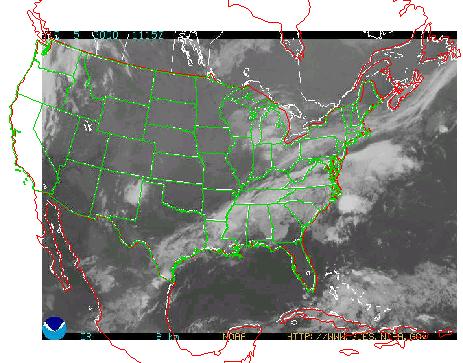
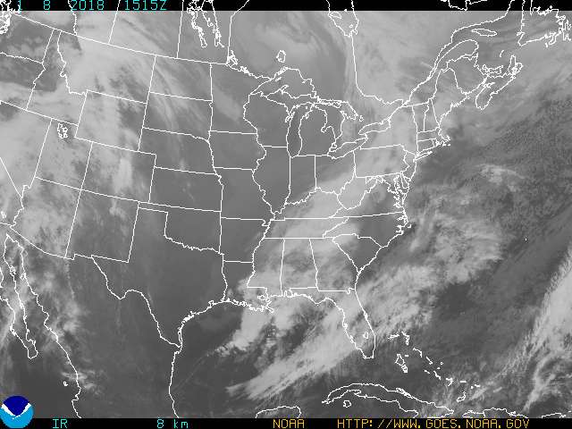
Figure 1: GIS registration to this NESDIS image section (5 Jun 2000 @1115Z) is excellent. The map
projection and registration are unpublished. To recreate this image with ArcView, get a fresh jpeg
from NESDIS at http://www.goes.noaa.gov/GIFS/ECIR.JPG. Set projection under
View Properties to Lambert Conformal Conic (under projections of the United States, custom) with
DATUM = WGS 84, Central Meridian = -88, Reference Latitude = 37, and Standard Parallels = 45,37.
Remember to enable the jpeg extension. Create a world file named ECIR.JGW with the following contents:

 8078
 0.0
 0.0
 -8043
 -2580000
 1930336
 

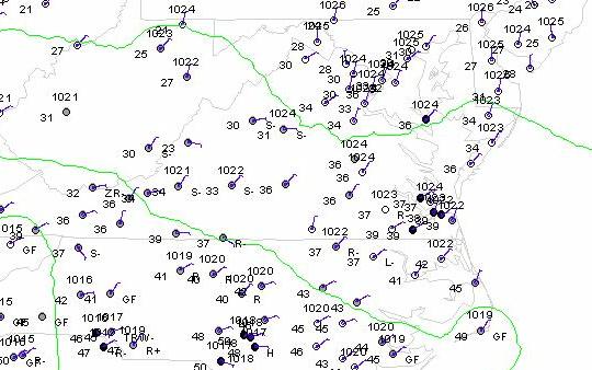
Figure 2: METAR surface observations at 1200Z (u.t.) on 12 Feb 2000 for Central East Coast.
Station locations are shown as dots, shaded to indicate reported cloud cover. Wind direction is
shown as a barb (from Weather Symbols palette in ArcView). Temperature [F], pressure [mb or hPa],
and significant weather are included as text. Pressure contours were created using Spatial Analyst.

Many correspondents have asked where "GIS-Ready" hydromet data are located on the internet. Our short list for "GIS-Ready" or "weather crypt" to GIS converters is given in Table 1. Many of these data are free or available from the Government at modest charge. Commercial sources are also available. DTN Kavouras announced GIS-Ready Weather Data services at the AMS Annual Meeting in January 2000!

Table 1: Where to get on-line weather data. Some of these are GIS Ready!
These URL's tested on 5 Jun 2000.

2.1 Rawinsonde Plotting Errors

It has been common practice to map rawinsonde data over the release points, even though the balloons have obviously drifted off, since horizontal displacement is considered small with respect to variation in hydromet data surfaces. However, consider the raob trajectories shown in Figure 3 for 1998 Dec 29, 12Z. Raob data from FSL archives at http://raob.fsl.noaa.gov/ were ingested as tables to GIS, corrected for quality problems, then used to calculate location during ascent. Location data is gathered during balloon ascent, but is discarded in the transmitted upper air message. Figure 3 shows a reanalysis (shaded contours) of the 100 hPa wind speed based on projected raob locations. The difference in resampled wind speed at the release points and "actual" positions is 5 m s^-1 in regions of strong vertical wind shear, most notably at the entrances and exits of jet streaks. This error level has been assumed to be a fundamental limitation of rawinsondes, but may be simply the result of poor sampling or analysis strategies. The same procedure can be applied for analysis of position errors impacting wind direction and even the temperature field. These errors are non-trivial and must be considered in current hydrometeorological practice. We further recommend that the geolocation information that has been discarded to save storage space be reinstated. The authors also note that GIS is a natural tool for raob quality control (QC), and lends itself to automation.

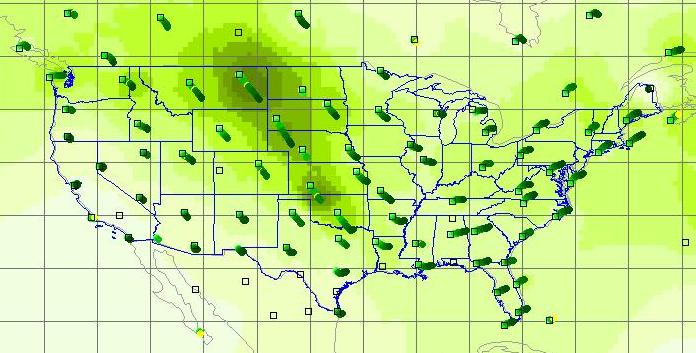
Figure 3: Rawinsonde tracks reveal extent of spatial offsets at higher altitudes. 100 hPa reanalysis by GIS demonstrates
a 5 m s^-1 sampling error if these obs are assumed to be located over the release point.

2.2 Overlaying Radar on Satellite Images

Spatial collocation challenges abound when combining radar data and satellite imagery. Consider the overlay of NEXRAD for Mobile, AL over the georeferenced NOAA-15 composite image for Tropical Cyclone (TC) Georges (1998 Sep 27, 2053Z) shown in Figure 4. This POES image was geolocated using visible surface features such as coastline and rivers. The NEXRAD reflectivity locations were calculated as polygons by ray tracing over the NAD83 ellipsoid (nex2shp.exe converter in Table 1). Nonetheless, the apparent eye locations are displaced by about 20 km, perhaps due to mislocation of the image "eye" through parallax (when viewed at an angle, high clouds are displaced in apparent location with respect to the surface), or image misinterpretation. The NEXRAD eye agrees with the position recorded by the NHC (question marks). The data in Figure 4 were prepared in support of the Open GIS Consortium (Sickels et al., 1999) Sep 10th demonstration of the Web Mapping Testbed. Most notably, the georeferenced satellite image was provided by Robert Fennimore of NESDIS, and is available on-line at the NOAA Operational Significant Event Imagery Server (OSEI, see Table 1).

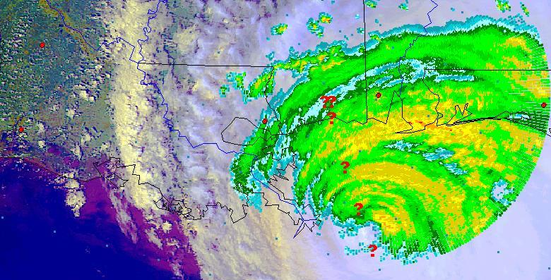
Figure 4: NEXRAD and NOAA-15 AVHRR eye positions for TC Georges are offset by 20 km. This NESDIS satellite image is registered very well to surface features including rivers and coastline.

3. Emerging Climate Applications
A first survey of GIS applications in climate and meteorology was provided by Shipley and Graffman (1999) at the 15th IIPS conference. That survey sited climate efforts at the Air Force Combat Climatology Center (AFCCC), see Rabayda (1998). Since then, the AFCCC has improved ArcView GIS capabilities for climatic data handling and report generation. For example, AFCCC analysts use Shapefiles of metadata about surface observations to manage that data and repositories in an Oracle DBMS to generate regional climatologies upon request. According to Michael Squires (personal communication), this GIS application has reduced the time needed to process large regions from several days to now in less than an hour. Other recent improvements include the Operational Climatic Data Summaries (OCDS) - four-page text documents of climatology information for about 5,000 sites. The OCDS library is loaded into Oracle DBMS and cross-referenced using GIS to generate new analysis products as needed "on the fly", or to generate input for a statistical model that uses this information as input. Another new GIS application uses tornado and hail event Shapefiles from the Storm Prediction Center (SPC) to serve requests for the frequency of severe weather.

Another exciting development for GIS is the acquisition this past year of ArcView GIS by the National Climatic Data Center (NCDC). NCDC is using ArcView GIS to develop a new climatic atlas (Plantico et al., 2000). Credit to C. Bruce Baker and especially Dick Cram at NCDC, for their encouragement in our development of the NEXRAD to Shapefile decoder (see Table 1). 3-D GIS analysis for NEXRAD data was first released by the lead author in an NCDC seminar in April, 1999, as shown in Figure 5.

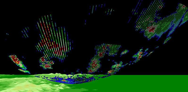
Figure 5: NEXRAD reflectivity as polygons in three dimensions. Sterling, VA NEXRAD data for 0.5 degree elevation angle is shown over a flat Earth with topography. These data are plotted as independent polygons with attributes for reflectivity [1-16 dBz] and height [m] using ArcView GIS with 3-D Analyst. GIS data structures will support radar ducting analysis on a radar cell-by-cell basis.

Another significant GIS/climate activity is the University of Oregon's Parameter-elevation Regressions on Independent Slopes Model (PRISM). Many climate variables are provided on-line as ASCII grid files, which can be downloaded to ArcView GIS with Spatial Analyst(TM). The PRISM site is located at http://www.ocs.orst.edu/prism/prism_new.html

4. Emerging Hydromet Applications

The majority of papers at the various conferences of the 80th Annual AMS Meeting which cite GIS in their abstracts are hydrometeorological applications. Applications of GIS in hydrology are too numerous to mention. However, a significant development this past year is the establishment of the Consortium for Developing and Implementing New GIS Capabilities in Water Resources, headed by David R. Maidment. A joint activity of the Center for Research in Water Resources (CRWR), University of Texas at Austin, and the Environmental Systems Research Institute, Inc. (Esri) , the initial focus of the consortium is on design of a new GeoDatabase Model for Rivers and Watersheds for ARC/INFO version 8, see http://www.crwr.utexas.edu/giswr/.

In addition, and as reported by Shipley and Graffman (1999), ArcView GIS has been obtained by all NWS WFO and RFC offices for local applications, including the maintenance of NWS map databases. Applications of GIS at the local offices have grown in number and scope, and were a contributing factor to the establishment of the NWS "GIS Forum" in 1999 (see section 4.1). Adoption of Arcview GIS by the WFO's led to substantial savings in LCC for the AWIPS program, and has resulted in the high-quality map databases for weather operations now in use by the NWS and commercial weather providers (see "Maps" in Table 1), also Vercelli (1999).

4.1 NWS@GIS Forum

The NWS convened its first ever GIS Forum at NWS Headquarters in Silver Spring, MD, June 30 - July 1, 1999, see Schultz and Reeves (1999). This event brought together a wide range of expertise, from forecasters to academics, to explore the benefit and applications of COTS GIS in NWS operations. For more on GIS@NWS, see http://www.nws.noaa.gov/om/gis/ . A good idea emerging from the GIS Forum was the realization that the AWIPS Local Data Acquisition System (LDAD) probably provided an excellent platform for COTS GIS installation and applications. It was also realized that there are no requirements established for COTS GIS in the NWS, nor are there personnel qualifications or job categories in the NWS which currently require GIS skill or training.

4.2 Meteorological Function Calculator (MFC)

The "Map Calculator" functionality provided in Spatial Analyst provides an interesting model for a "Meteorological Function Calculator" or MFC, supporting a general interactive capability to perform typical and some highly esoteric transformations of gridded hydromet data. The concept for an MFC is shown in Figures 6-8, starting from a registered model grid in Figure 6, and ending with derived GRID calculations in Figure 8. To avoid confusion in terms, we will use lower case 'grid' to denote any numerical model grid field as commonly understood by meteorologists. We then use upper case 'GRID' to identify the Esri GRID layer. Figure 6 shows a model grid layer (NGM surface temperature) registered to a Polar Stereorgraphic projection. Since the various model grids do not change location, the registration files can be set up once and the various (Esri) GRID layers can be exchanged as desired. Users then invoke the MFC to create and simplify hydromet calculations.

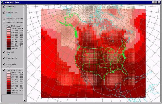
Figure 6: Gridded surface temperature field from the NGM numerical model in Polar Steroegraphic projection. Also shown is a shapefile for the gridpoints of the NCEP ETA model. When registering gridded model data, it is useful to display surface height [gpm] from model layers, if provided, to verify that the grid has not been reversed, inverted, or otherwise mislocated.

A prototype of an MFC is shown in Figure 7. While still under development, this MFC functions very much like the Spatial Analyst Map Calculator, and demonstrates that ArcView users can manufacture cool stuff like this on their own. Basically, available GRIDs are listed including MFC products in a GRIDs window, identifying the root model (e.g. ETA), the GRID parameter or field (e.g. HGHT, TEMP, ...), the GRID layer level (typ. 1000, 950, 900, ... [mb or hPa]), and GRID valid time (e.g. 0 for 0000 u.t., 12 for 1200 u.t.). Typical calculations such as the geostrophic wind (which is derived from a layer height field at constant pressure, or a pressure field at constant height, or a Montgomery Stream Function in isentropic coordinates) are established with buttons of their own (e.g. 'Wind' in Figure 7). An equation involving the GRIDs is developed similar to an Avenue statement as the user selects GRIDs and operations, including the Gradient (Del), Laplacian (Del^2), and Divergence (Del dot). The goal is to provide a unified user interface that looks like common hydromet practice, while taking greatest advantage of the intrinsic ArcView functionality. We have concluded that model GRIDs need to be associated in time as a set of GRIDs (e.g. p, T, q, u, v, ...), since many hydromet calculations combine these various parameters for a given valid time. Time derivatives look for GRID sets organized by hydromet parameter.

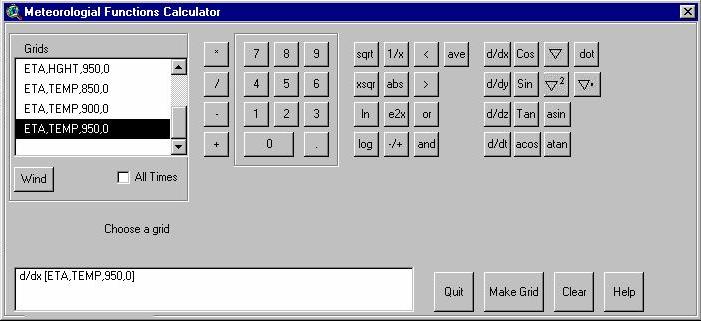
Figure 7: Application of the MFC to calculate a derivative with respect to the x-axis. In the case of a polar stereographic, note that the x-axis does not align with parallels except at the central Meridian (105 W in Figure 5). Distance for the derivative must be calculated at each location. For lat/lon grids (see Figure 8), distance is a function of latitude and changes only along the y-axis.

The logical conclusion is to create derived GRID fields from available grid field information. The global MRF model is used to demonstrate calculation of the geostrophic wind as shown in Figure 8. The MRF is a 1 degree lon/lat model, providing analysis and forecast information from -180 (West) to + 180 (East), and from +90 (North) to -90 (South). Once the surface height field was registered to verify collocation, then the 850 hPa layer (850 mb surface) was used to calculate V_g, which combines the pressure gradient or height gradient at constant pressure with the "Coriolis" parameter (rotation rate of the Earth), air density, and gravity to produce an estimate of wind speed assuming no drag due to friction with the Earth's surface. This calculation was compared to the MRF grid for geostrophic wind for verification, and they were identical. Other parameters calculated and so verified include absolute and relative vorticity, and divergence. The 3-D Analyst was used in Figure to view the results and produce Figure 8, illustrating the nature of "lows" and "highs" on an 850 mb surface. In addition, GRID points that were below MRF surface pressure were removed from the GRID as voids, allowing the GIS meteorologist to visualize and prepare for flow around rather than through mountains.

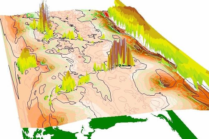
Figure 8: East-West component of geostrophic wind on 850 mb [hPa] height surface from the MRF global model (1-degree lon/lat resolution). 3D-Analyst is used to show topography of the 850 mb surface. A global terrain model is included to show where the 850 hPa surface is below ground.

5. What's Next?

What we're really waiting for is the universal adoption of GIS-Ready or even GIS-friendly formats for hydromet data. DTN Kavouras is the first commercial source to provide comprehensive GIS-Ready data services. Other commercial and even public data services may still consider proprietary formats as a clever strategy to acquire and maintain market share in the hydromet niche. Today, the data source organization has the option to provide data in formats of their choice and at their discretion, in accordance with the so-called Golden Rule. These formats are subject to change without notice, are mutually incompatible in most instances, and require special purpose programs or translators to display and/or transform them to your platform. Strategies such as Hierarchical Data Format (HDF) specify a metadata format, but do not actually specify the data format per se. Instead, HDF users must acquire libraries of data format conversion algorithms which are called when needed. Just how expensive are these libraries and how difficult will they be to maintain? Will they be GIS-Ready?

In the case of METAR data (surface observations), a comma delimited format has been suggested that supports insertion into Excel as well as ArcView GIS. This format is ideal for most systems. A comparison for comma delimited ingest among Intergraph, MapInfo, Atlas, and ArcView was favorable, with ArcView providing the greatest flexibility in interpretation of the null field value (i.e., ArcView was most consistent with Excel). RAWINSONDEs would benefit from a transition to a comma delimited format, although the trend today in the University community is to adopt the NetCDF standard.

NEXRAD radar data should become available publicly with the dissolution of the NIDS contracts by October 2000. Once released from the proprietary interests of the NIDS contractors, these data should be available in near-real-time on the internet. Converters such as nex2shp.exe and dpa2shp.exe (see Table 1) will probably be the procedure of choice, since NEXRAD level 3 products are efficiently packed, whereas Shapefiles for the same information are enormous.

Hydromet images are abundant on the internet (e.g. http://iwin.nws.noaa.gov/). These images are provided in diverse projections, each of which can be readily incorporated into a GIS View. However, we note that there are many projections in use, making it harder to combine the information provided in related images. Information of interest include model gridfields as GRIB, DIFAX charts as TIFs, and geolocated satellite images as GIFs, TIFs, and JPGs. Would it be too much to ask for a just a little more standardization?

6. Acknowledgments

The authors wish to acknowledge the support and efforts of Mike Heathfield, Robert Reeves, Roger Shriver, David Vercelli, and Pat Welsh of the National Weather Service, and the Department of Geography, George Mason University. Additional contributions and suggestions were received from Keith Jenkin (TRW), Ron Sznaider (DTN Kavouras), John Sherwood (The Weather Channel), Steve Sickels (Open GIS Consoritum, SECON), Robert Fennimore (NESDIS), C. Bruce Baker, Howard Carney, and Richard Cram (NCDC), David Maidment (U. Texas), Demos Christodoulidis (Raytheon ITSS), Al Peterlin and Ray Motha (USDA), Michael Squires (AFCCC), and last but not least Karen Singley (formerly of GMU and Raytheon) and David Beddoe of Esri.

7. References

Dana, P.H., 1994: Geodetic Datum Overview; http://www.utexas.edu/depts/grg/gcraft/notes/datum/datum.html

NWS, August 1999: Interface Control Document for AWIPS - NESDIS (NOAAPORT ICD, section 4.7); http://www.nws.noaa.gov/noaaport/html/refs.shtml

Plantico, M.S., Goss, L.A., Daly, C., and G.H. Taylor, 2000: Development of a New U.S. Climate Atlas. 11th Symposium on Global Change Studies, Paper P1.12, AMS Annual Meeting, Long Beach, CA (Jan 9-14).

Rabayda, A.C., 1998: AFCCC Applications of ArcView GIS and ArcView Spatial Analyst. Esri International Users Conference, Paper 450; http://www.Esri.com/library/userconf/proc98/PROCEED/TO450/PAP450/P450.HTM

Reeves, R.W., and J.R. Schultz, 2000: IOS Paper 2.10, Development of a User-Friendly, Interactive Web Guide to in situ Observing System Metadata using GIS Technology; http://obsystem.nws.noaa.gov

Schultz, J.R., and R.W. Reeves, 1999: GIS@NWS Forum for the Discussion of Applications and Requirements for Geographic Information Systems (GIS) at the National Weather Service, Silver Spring, MD, 30 Jun - 1 Jul; http://www.nws.noaa.gov/om/gis/

Shipley, S.T. and I.A. Graffman 1999: GIS Meteorology. 15th IIPS, Paper No. 16.8; http://geog.gmu.edu/projects/wxproject/papers/15iips/15iips.htm

Sickels, S. ,et al., 1999: Open GIS Consortium demo of The Web Mapping Testbed, Phase 1; http://www.opengis.org/wmt/

Vercelli, D., 1999: Developing Standard GIS Functionality, A Model for Field/Headquarters Synergy. GIS@NWS Forum, http://www.nws.noaa.gov/om/gis/standard/standard.htm

Dr. Scott Shipley (Scott_T_Shipley@Raytheon.com) is also an Associate Professor with the Department of Geography, George Mason University, sshipley@gmu.edu, http://geog.gmu.edu/projects/wxproject.

Ira Graffman (Ira.Graffman@noaa.gov) and Joseph Ingram (Joseph.Ingram@noaa.gov) are currently assigned to the AWIPS Program at the National Weather Service, http://isl715.nws.noaa.gov/mapdata/.