Winter flood flows in the eastern desert of Jordan represent a potential source of water that could be developed to satisfy the local needs. The lack of reliable estimates of flow records in the area stands as a barrier in front of developing successful water harvesting schemes. This paper describes a simplified surface water model that can be used to generate the required flow records. The model applies GIS techniques to describe the catchment topography and the active hydrological processes as well as to simulate the runoff generation and routing processes.
A hydrological model is a simplified simulation of the complex hydrological system. The major problem in modeling the hydrological processes based on their physical governing laws is the variability in space and time of the parameters that control these processes (Porter and Mcmahon, 1971). In the first generation of hydrological models this has been dealt with by assuming homogeneous properties for the hydrological processes over the whole catchment area or, in the best cases, for subdivisions of the catchment area ( Moore et al, 1993).
Over the last twenty years the need for hydrological models has shifted from generating stream flow hydrographs into predicting the effects on water resources of the actual land use practices (Abott et al, 1986) or the need to estimate the distributed surface and subsurface flows (Moore et al, 1993). These needs require better description of the catchment topography and the distributed properties of the hydrological processes acting on it.
With the emergence of remote sensing techniques as potential sources of data of the hydrological processes and the improved capabilities of generating and processing DEM data, GIS techniques have gained a prominent role in hydrological modeling. This role has developed from the traditional use of GIS as an interface to the hydrological models for pre-processing and post processing of data into "rethinking hydrological models in spatial terms so that better GIS-based hydrological models can be created" (Maidment, 1993).
This paper presents a simplified GIS-based hydrological model (WR-model) used to generate runoff records for Wadi Rajil watershed, an un-gauged arid catchment in Jordan.
The model is composed of two components: the runoff generation component and the flow routing component. Each component consists of a group of functions representing the hydrological processes involved in the circulation and distribution of the surface water within the catchment (figure 1).
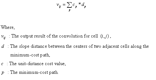
The raster data model used to simulate the hydrological processes involved reflects the distributed nature of these processes. The model computations are carried out on cell-by-cell bases for each time step of the input rainfall event using the following water-budget equation:
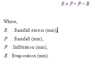
This formula assumes no base flow contribution to the runoff. This is mainly due to the fact that the depth to the water table in most of the catchment area exceeds 100 meters.
The rainfall excess generated at each cell will be routed to the watershed outlet by the functions of the flow routing component. The flow routing process can be simulated by tracking the rainfall excess from cell to cell to the watershed outlet (Olivera and Maidment, 1996). The detailed description of the tracking process involves complex flow dynamics equations. The WR-model applies a simplified approach based on the following assumptions:
1. The rainfall excess generated at each cell flows out in one direction along the steepest slope.
2. The routed cell flow does not interact or affect any flows from other cells sharing the same flow path (Olivera and Maidment, 1996).
Under these assumptions the flow routing process is simulated as a combination of two grid layers:
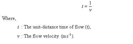
1. The time-of-flow grid representing the time required for the runoff generated at each cell to reach the outlet. This grid can be produced using the FLOWLENGTH function that carries out the following convolution computations:
By manipulating the cost values the function can be used to perform any sort of convolution required. Olivera and Maidment (1996) have reported such an application for a cell-based routing application using the diffusion wave model. Therefore, if we consider the time of flow as the unit-distance cost value of the cost grid then the FLOWLENGTH function can be used to generate a grid layer representing the time required for the flow at each cell to reach the watershed outlet. The unit-distance cost value can be expressed as follows,
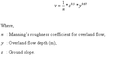
Assuming fixed flow velocity of 1 for the channel cells and variable flow velocity (V ) for the overland flow cells a grid layer showing the distribution of flow velocity over the catchment can be calculated. The overland flow velocity (v) can be computed from the following formula of Mannings;
2. The discharge grid. The flow routing is simulated as a pure translation process that assumes no abstractions due to storages over the flow pathway. However, the model considers the significant influence of the transmission losses on the routed flows by subtracting these losses from the discharge contributed by each cell at the watershed outlet. The transmission losses are computed based on the following formula (Jordan, 1977).
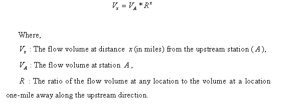
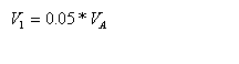
The study of Walters (1990) on transmission losses in Saudi Arabia has shown that the transmission loss (V1) at 1 mile from the upstream station is given by the following regression equation;
Using the FLOWLENGTH function the transmission losses for each cell can be calculated. The discharge grid is produced by subtracting the transmission losses from the rainfall excess amounts calculated by the first model component. The methodology used to generate a hydrograph at the watershed outlet can be outlined as follows:
1. For each time step of the input rainfall event two grids are generated; the isochronal grid and the total discharge grid. The isochronal grid is produced from a classification of the time-of-flow grid according to the required time step of the hydrograph. The resulting isochronal grid is then used as a parameter to the ZONALSUM function to produce a grid representing the total discharge contributed by each isochrone.
2. By merging the two grids, the isochronal and total discharge, a new grid is produced that includes both attributes, the time of concentration and the total discharge, for each time zone. This grid represents the catchment response corresponding to one time step of the input rainfall event.
3. The final hydrograph corresponding to the rainfall event is generated by shifting in time the hydrograph of a given input time step over that of the previous time step and summing up the values according to the specified hydrograph time step.
The model was used to generate hydrographs for the catchment area of Wadi Rajil, a major catchment area in the eastern arid part of Jordan. The watershed area is about 2812 that drains most of the ephemeral wadis in the area. Most of the area is covered by basalt stones and characterized by the presence of many mud flat areas. Rainfall events in the area are in general of high intensity, short duration and high spatial and temporal variability. The long-term annual average of rainfall is 71.5 mm.
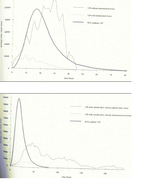
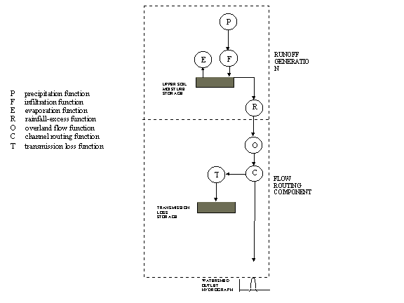
The model has been used to generate unit hydrographs under different combinations of flow velocity and transmission losses. The first hydrograph, shown in figure (1), was produced assuming fixed flow velocity and no transmission losses.
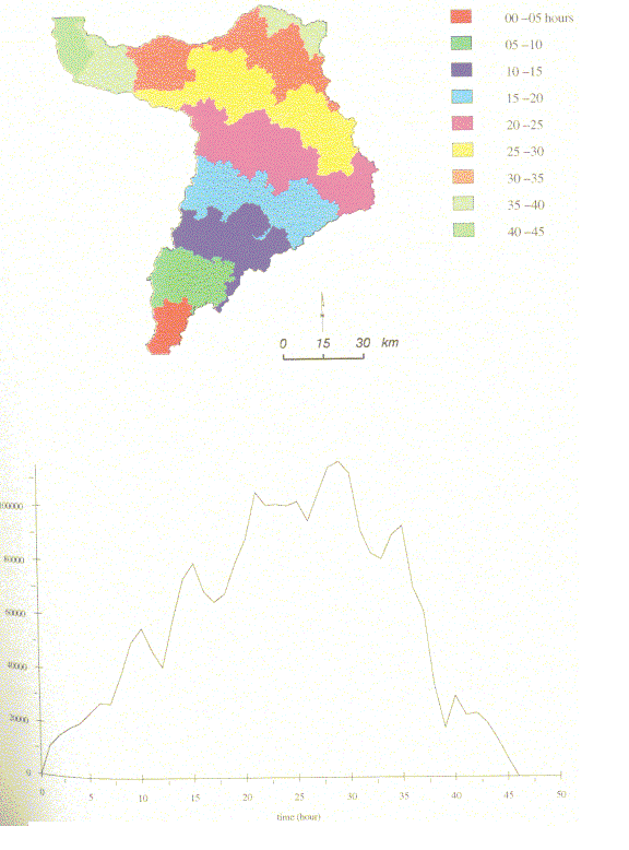
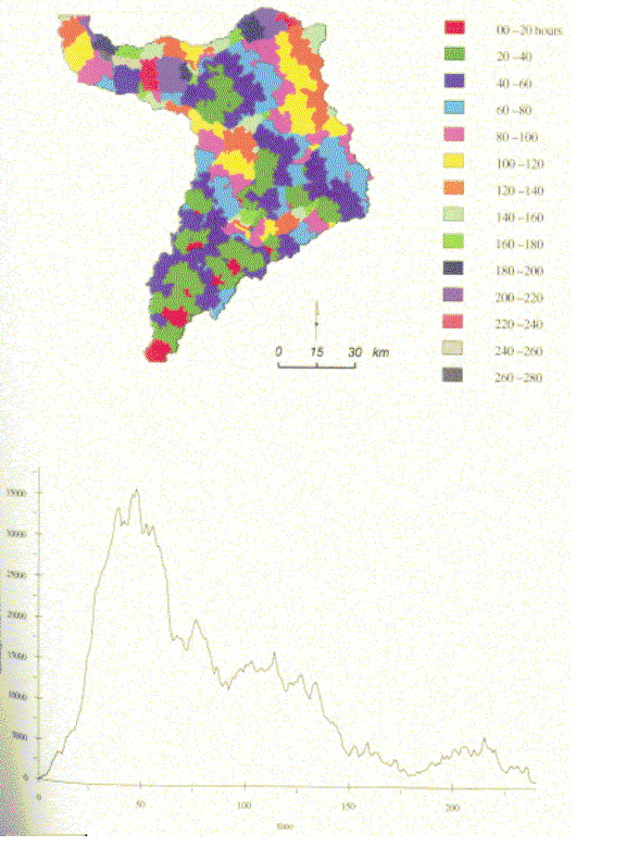
These assumptions comply with the unit hydrograph theory, which assumes constant time base of the hydrograph and no abstractions of the routed amounts. The constant time base of the unit hydrograph implies that, for a given cell location, the time of travel to the watershed outlet, and hence the velocity of flow, is the same for all rainfall excess amounts (Maidment, 1993). The hydrograph has steep rising and falling limbs and a relatively short time of concentration of about 1.5 day. The isochrones shown in the figure exhibit distinct zones of relatively uniform shapes and regular distances from the outlet. Figure (2) shows a hydrograph generated assuming variable overland flow velocity. The hydrograph has a steep rising limb but relatively longer recession period. The isochrones reflect the effect of slope on the velocity of flow and hence the time of concentration. For example, the upper north west area has shorter time of concentration than areas to the north which are geographically closer to the outlet.
As shown in figure (4), the unit hydrograph generated under fixed flow velocity and
no transmission loss shows relatively good fit, in terms of the peak flow and time to
peak, with the SCS unit hydrograph. This implies that previous estimates of the
discharge of Wadi Rajil based on the synthetic unit hydrograph (the SCS unit
hydrograph) may have not included the influence of transmission losses.
The raster data structure and the raster processing functions have been used to represent the hydrological processes and their interactions in a distributed modeling approach. Two raster-processing functions proved to be very useful tools for hydrological modeling. First, the FLOWLENGTH function that can be used to carry out any convolution processes involved in simulating complex hydrologic and hydraulic flow routing procedures. Secondly, the COMBINE function was used to produce a hydrograph grid by carrying out a spatial merge of the isochronal and total discharge grid layers.
Abbott, M., Bathrust, J., Cunge, J., O'Connell, P. and Rasmussen, J. (1986) An introduction to the European Hydrological System-Systeme Hydrologique Europeen, "SHE", 1 : history and philosophy of a physically-based, distributed modelling system. Journal of Hydrology, 87, 45-59.
Abbott, M., Bathrust, J., Cunge, J., O'Connell, P. and Rasmussen, J. (1986) An introduction to the European Hydrological System-Systeme Hydrologique Europeen, "SHE", 2 : modelling system. Journal of Hydrology, 87, 61-77.
Environmental Systems Research Institute. (1996) Cell-based modelling with GRID. Esri, California.
Jordan, P. (1977) Streamflow transmission losses in Western Kansas. Journal of Hydraulics Division, 103(8), 905-919.
Maidment, D. (1993) Developing a spatially distributed unit hydrograph by using GIS. In : Applications of GIS in hydrology and water resources (edited by Kovar, K. and Nachtenebel, H.) Proceedings of Vienna conf., April 1993. IAHS publ. no. 211. 181-192.
Maidment, D. (1996) GIS and hydrologic modeling-an assessment of progress. Internet : http://www.ce.utexas.ed...1/maidment/santafe.html.
Moore, I., Grayson, R. and Ladson, A. (1993) Digital terrain modelling: a review of hydrological, geomorphological and biological applications. In : Terrain analysis and distributed modelling in hydrology (edited by Beven, K. and Moore, I.). John Wiley & Sons, Chichester.7-30.
Olivera, F. and Maidment, D. (1996) Runoff computation using spatially distributed terrain parameters. Internet: http://ciil.ce.utexas...dro/olivera/ASCECA1.HTM.
Porter, J. and McMahon, T. (1971) A model for the simulation of streamflow data from climatic records. Journal of Hydrology, 13, 297-324.
Walters, M. (1990) Transmission losses in arid regions. Journal of Hydraulic Engineering, 116(1), 129-138.