The problem of finding the optimal allocation of wetlands is approached from an evolutionary viewpoint using a genetic algorithm. Two different and spatially dependent wetlands are allocated along a network of polluted streams in the Skjern Ĺ delta, which is located in the western part of Denmark. The objective is to minimize the operations costs of such wetlands and minimize deviations from stated [Fe2+], which are suitable for salmon habitat. The stream-order and the wetland-order influence the feasibility space and restrict the traditional transition operators such as crossover and mutation. It is shown that the algorithm finds near-optimal solutions in a reasonable number of iterations. A GIS-modeling environment is supplied with these static solutions and the dynamic effects are modeled.
Keywords: Genetic algorithms, geographical information systems, optimization.
Landscape planners are increasingly confronted with legislative demands to plan and design solutions for complex spatial and temporal problems in the landscape through different types of impact assessments. Solutions to any given location problem has an infinite number of solutions where the challenge is to find the most optimal solution based on a set of criteria (Steinitz, 2000).
As an example mitigation and restoration of wetlands represents a complex and long-term spatial problem. Location as well as sequences of wetlands along riparian zones in the watershed is of importance (Mitch, 1992) where wetlands poorly located might act as sources instead of sinks thus polluting further downstream. Also mitigation and restoration is performed with constrained budgets where optimal. While feasible solutions in large scale based on expert judgment might easily be sought some excellent solutions in smaller scale may be missed. Based on this argument Chiang et.al. (1977) implements a heuristic algorithm to optimize the location of wastewater treatment plants.
Genetic algorithms (GA) belong to a class of algorithms termed evolutionary computation, which also includes evolutionary programming, evolutionary strategies, and genetic programming. A review of the history is presented in, e.g. Bäck (1996). They are population oriented and use selection, mutation, and recombination operators to generate new solutions in a search space.
Since wetlands represent complex systems with high level of spatial and temporal interactions where objectives often conflict the allocation should be based on multiple criteria evaluation. This paper uses a genetic algorithm embedded in a GIS environment to solve this allocation problem.
Section 2 contains the allocation problem. The dynamic modeling system is described in Section 3. An introduction to the genetic algorithm is provided in Section 4. The results of the experiments on using the genetic algorithm to solve the problem including a pre-optimization of the parameter settings, and the dynamic modeling are presented in Section 5. A discussion and conclusions are given in Sections 6.
Due to agricultural drainage in extensive farming areas, open pit mining and geological structures of the Western part of Jutland, Denmark many streams are polluted with precipitated iron hydroxides primarily ochre (Fe(OH)3). In recent years wetlands has been reintroduced as a long-term low cost effort to facilitate and re-mediate precipitated ochre. Reintroducing wetlands in riparian areas concentration of ferrous iron (Fe2++) and pH are among the key determinants for ochre precipitation processes and retention time for the remediation processes. Two different kinds of wetlands may be located along the streams to increase the water quality of the system.
The planning objective is to minimize the costs of operating such wetlands and minimize deviations from stated [Fe2+], which are found suitable for salmon habitat. The problem is based on real water quality data as well as realistic objectives. The watershed is modeled as grid cells, and each cell is connected to at least one up stream and down stream cell. Altitude, stream flow and water content are modeled in the system.
Let c denote a specific cell in the stream and let C represent the stream configuration of the whole Skjern Ĺ delta. Each cell ![]() may be used in different ways. Considering the choice of wetlands we let D denote the possible decision alternatives in each cell, and
may be used in different ways. Considering the choice of wetlands we let D denote the possible decision alternatives in each cell, and ![]() denotes the specific alternative picked for cell c. In the problem each cell may be seeded with three different wetlands, and therefore D={no wetland, wetland-A and -B}. A specific allocation configuration of wetlands along the stream can be denoted as . Additionally, let denote the resulting water quality of ferrous iron in each cell configuration.
denotes the specific alternative picked for cell c. In the problem each cell may be seeded with three different wetlands, and therefore D={no wetland, wetland-A and -B}. A specific allocation configuration of wetlands along the stream can be denoted as . Additionally, let denote the resulting water quality of ferrous iron in each cell configuration.
The planning decision, that the local community faces, is the one of obtaining a certain level of water quality without violating a budget constraint. The construction and maintenance costs of each type of wetland vary depending on size. Usually, more wetlands increase water quality. However, some upstream configuration may in fact reduce the effects of some downstream configurations towards zero. Hence, some logic rules to test this assumption could be implemented.
The stated objective is to minimize the overall value of the wetland configuration represented by costs subject to water quality represented by maximum [Fe2+] for all ![]() . The mathematical formulation of the problem for the whole stream is expressed as maximizing the number cells with improved deviations from
. The mathematical formulation of the problem for the whole stream is expressed as maximizing the number cells with improved deviations from ![]() :
:
subject to the stated, the financial constraint is formulated as:
where ![]() represent threshold values of [Fe2+] for each cell in the stream. In the following we will give some real content to (1) and (2).
represent threshold values of [Fe2+] for each cell in the stream. In the following we will give some real content to (1) and (2).
The wetland transformation model presented here consists of a hydrological model (HYM) and a chemical transformation model (CTM) for the oxidation, hydrolysis and precipitation of ochre.
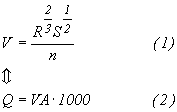
From sample stations along rivers Q is interpolated for each 25 m's by combining surface- and subsurface flow accumulation grids as key index for interpolation. Using Newton iterative approach combing (1) and (2) and knowing width, slope (S) and estimating Manning's quotient for kinematics' friction (n) V is calculated for each 25 m of the stream.
Three key processes determine the transformation of ferrous iron into ochre: Oxidation, hydrolysis and precipitation of ochre altogether being net acidic for the wetland. Oxidation happens either biotic or abiotic following the same stocheometric process:
The rate of oxidation can be expressed as:
where k is the oxidation constant, [Fe++] the concentration (mg/l) of ferrous iron, pO2 partial pressure of oxygen and pH. Oxidation rate below pH 4.5 is increased by a factor105 due to biotic oxidation. Hydrolysis is referred to as being only abiotic following the equation.
Hydrolysis and precipitation of ochre from ferric iron is defined from the relation between solutability product constant (KFe(OH)) and the product between the ion constants (QFe(OH)). For each moles of ochre three moles of H+ is released why transformation without HCO3- buffering creates net acidic conditions in the wetland. The main buffering comes from bicarbonate:
From 7 Danish wetlands the average construction cost for sedimentation basins range from 63 - 295 dkk/m2 and yearly maintenance from 1 - 23 dkk/m2. For vegetated wetlands an average construction costs is 30 - 100 dkk/m2 and the yearly maintenance range from 0 - 20 dkk/m2.
The algorithm operates on a population ![]() of l individuals for each generation g. From the initial population subsequent populations P(1),..,P(g) will be computed by employing the three genetic operators of selection, crossover, and mutation. After calculating the fitness value
of l individuals for each generation g. From the initial population subsequent populations P(1),..,P(g) will be computed by employing the three genetic operators of selection, crossover, and mutation. After calculating the fitness value ![]() , a mating pool is formed by selecting the more fit individuals.
, a mating pool is formed by selecting the more fit individuals.
A general formulation of the procedure involves the following steps:
The selection is based on tournament selection (Baker 1985, Goldberg 1989, Goldberg and Deb 1991). During the mating some individuals are transformed by mutations, which create new individuals by a small change in the individuals' binary structure or by crossover where parts of two or more individuals are combined. A feasible initial solution for the first generation is obtained by randomly assigning one of the alternatives in D to a randomly defined stream segment without violating the budget constraint. In the following, the fitness function, genetic operators and the selection method applied by the GA are presented.
The fitness formulation (eq.1 and eq.1.2) is not used directly as a fitness measure for each stream string. Instead each configuration/solution is given a new fitness value according to its order in the population based on the objective function value.
From eq.1.1 FFe(F(c,d( C))) can be stated as follows:where FFe is the rate of cells c below ![]() . The constraint on construction and maintenance costs is expressed as:
. The constraint on construction and maintenance costs is expressed as:
where fmax represents the threshold cost value. The closer f(c,d(C )) is to fmax the smaller the value. Combining eq.4.1 and eq.4.2 the fitness values for each solution i are given as:
Each member l of the population P is ranked ascending to Fi and assigned an accumulated probability value determined by its contribution to the total sum of the fitness values of l in the population Pg.
The parents, i.e. individuals, which survive the selection process, undergoes the genetic operations, mutation and crossover. Bäck (1996) and Goldberg and Deb (1991) conclude that in terms of selective pressure, tournament selection seems to be superior to ranking and proportional selection. Booker (1987) and Eshelman et al. (1989) find that an increasing number of crossover points may improve the performance of GA.
From a random generator Y(1,P) two members ln and ln+1 from Pg are selected from a mating pool where F(c,d(C )) 0. Two random numbers Y(1,C) and Y(1,6) are drawn to determine the crossing site and size of the crossing string. A crossover between the two individuals is then performed. From the mating pool the procedure is repeated until the number of individuals l equals the size of the population P.
Mutation occurs if a random value reaches a certain threshold. The random generator selects an individualUsing Arc Info version 7.2.1 (NT and UNIX) a genetic algorithm structure were implemented with an ochre transformation model using AML. To test the optimization algorithm two types of analysis were performed. In the first analysis an expert opinion were given to locate type, size and sequence of wetlands in the riparian zones of the catchments area. The 'rule of thumb' locates the plants as near as possible to the known source of pollution. In the second analysis the same wetland parameters were incorporated into the genetic algorithm.
The data was prepared for a small sub-catchments area of the Skjern Ĺ river delta with high rates of point and non-point pollution from ferrous iron. A 25 m grid of the streams was created and water quality parameters generated through interpolation based on a distribution from cell accumulation from surface and subsurface hydrologic flows.
The purpose with the data set was to test the behavior of the genetic algorithm why the data set was calibrated to fulfill this purpose. The calibration was performed using the ochre transformation model (section 4) to stabilize each cell based on in- and output rates. Table 5.1 illustrates the calibrated stabilized data. Both pH and HCO3- were kept as constants since the ochre model showed to be very sensitive to small changes in the pH level. Measurements from 10 Danish wetland systems for ochre remediation showed no noticeable drop in levels of pH and HCO3- when entering and leaving the two types of wetlands why this assumption presently seems valid.
The maximum construction and maintenance cost for the first year is set to 220.000 dkk. (~27.500 $US). Two types of wetlands were introduced: sedimentation basins and vegetated basins. The input parameters for both wetlands were (cell length = 25m):
| Sedimentation basin | Vegetated wetland | |
| Depth (m) | 0.70 | 0.25 |
| Wideness (m) | 30 | 30 |
| Construction (dkk/m2) | 131 | 13 |
| Maintenance (dkk/m2) | 100 | 20 |
| Total cost (dkk) | 108.000 | 90.000 |
Threshold value was set to 1.55 mg/l and maximum cost fmax to 220.000 dkk.
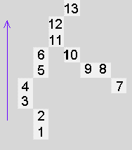
When source of pollution is known, experience locates remediation plants closest to the source. From Table 5.1 cells 1 and 7 are the most likely candidates for locating a wetland due to the high concentrations of ferrous iron.
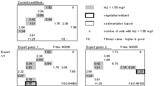
The numbers in the cells represents the concentration of ferrous iron with shaded cells showing values below the threshold. The 1/1 notation to the left indicates 1 individual with 1 generation. Current conditions, shows 6 cells out of 13 are below threshold value. Locating a vegetated wetland in cell 1 raises the number below threshold value to 8, where the wetland cell and its neighbor are improved. Locating the same type of wetland in cell 7 maintain the 6 cells below threshold. Cells 7, 8 and 9 are improved and cells 10, 11 and 13 are raised to values above threshold. Both solutions represent minimized costs.
Two runs were performed with the first run having 50 individuals in a population and 60 individuals in the second. Both runs were set to 5 generations since tests showed near optimal solutions after 5 generations for this subset of the watershed. In the first generation each individual were only allowed to have one wetland. Through mutation, over cross and selection the number of wetlands can increase.
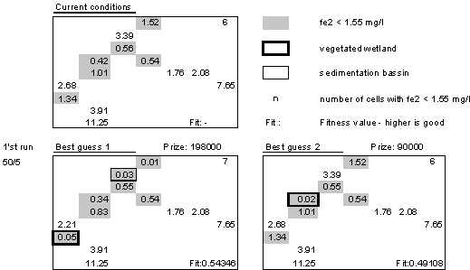
The best guess from the first run shows a vegetated wetland located in cell 3 and a sedimentation basin in cell 12. The number of cells below average is 7 with one of the wetlands located in a 'good' cell (3). Cost is relative high but within the given maximum prize. The second best guess locates a vegetated wetland in a 'good' cell not changing this solution from the current conditions.
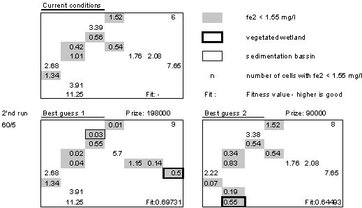
The second optimization run with 60 individuals has its best guess with two wetlands: a vegetated in cell 7 and a sedimentation basin in cell 12 giving 9 cells below threshold value. Costs are within the limits. The second best guess locates a vegetated wetland in cell 7 parallel to the best expert guess.
From the fitness values in the lower right corners the best solution also has the highest fitness value suggesting that the GA converges towards a near optimum solution. Plotting all accumulated cost values against number of clean cells indicates that the GA in the second run has visited the expert solution 1 and 2.
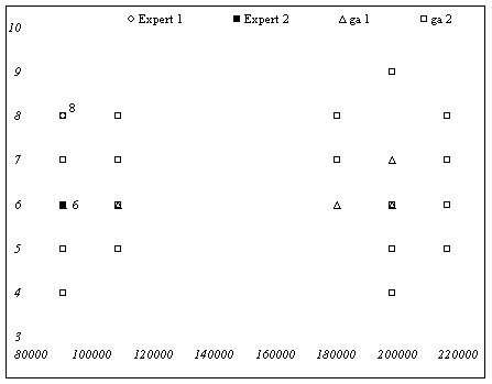
Fig5.1. The fitness values for all suggested individuals in the last generations plotted against the number of clean cells reveals that the GA second run has visited the two expert suggestions.
From the initial two tests the genetic algorithm showed capable of performing an optimization but only during the second run. In the first run it missed the near optimal solutions. Initial test runs revealed that the GA quickly stabilizes itself around optimums in the visited search space. If the search space hasn't been visited near optimum during the generation of a population selection and over crossing will not be able to reach that part of the search space. Only through mutation can the GA reach this part of the search space. The number of initial individuals therefore seems quite important and should be set sufficiently high. Similar high rates of mutations will improve the search. In these simulations the chance of one individual mutating were 10% in each generation with no mutations occurring during the test runs suggesting that this value should be increased with low numbers of generations.
Locating one wetland in the data set gives 13 possible sites. Locating any number of wetlands under a given financial constrain with the chosen wetland dimensions and costs presents 495 possible combinations rapidly adding to the complexity of the problem.
As seen in the second best expert guess these systems are dynamic non-linear systems where one improvement upstream caused downstream problems (a pattern revealed through other simulations). Through optimization the over all best GA guess indicated a possible solution to this problem. By doing so the GA suggests a near optimal solution in the solution space and thus aiding the decision making process on where, in what sequence and with what feasible consequences wetlands could be located.
The enemy number one to this approach is processing time. The time used for this simulation was approximately 35 minutes for each generation with 60 individuals, running on NT40, 400MHz Intel xeon processor. Increasing the size of the watershed will cause the processing time to increase >> n2, why guided search might be an option. One way to improve the search in the search space is to visit only those cells where problems occur. In the given case only visiting cells above threshold values. Another option is to reuse some of the previous calculations since the GA during its optimization approaches a near optimal solution consisting of relative identical strings in the stream network.
Bäck, T. 1996. Evolutionary Algorithms in Theory and Practice. Evolution Strategies, Evolutionary Programming, Genetic Algorithms. Oxford University Press, Oxford, 314 p.
Baker, J.E. 1985. Adaptive selection methods for genetic algorithms. In J.J. Grefenstette (ed.). Genetic algorithms and their applications. Proceedings of the second international conference on genetic algorithms. Lawrence Erlbaum Associates, Hillsdale, New Jersey, pp. 101-111.
Bjornsson, C. 1999. Approach to Dynamic Wetland Modelling in GIS, in Geographic Infrmation Research Trans-Atlantic Perspectives ed. Craglia M and Onsrud H, Taylor and Francis, pp. 203-217
Booker, L.B. 1987. Improving search in genetic algorithms. In L. Davis (ed.). Genetic Algorithms and Simulated Annealing. Morgan Kauffmann, Los Altos, California, pp. 61-73.
Chiang, H C and Lauria D T, 1977, Heuristic Algorithm for Wastewater Planning, Journal of The Environmental Engineering Division, Oct. 1977.
Eshelman, L.J., R.A. Caruana and J.D. Schaffer 1989. Biases in the crossover landscape. In J.D. Schaffer (ed.). Proceedings of the third international conference on genetic algorithms. Morgan Kauffmann, San Mateo, California, pp. 10-19.
Goldberg, D. 1989. Genetic algorithms in search, optimization, and machine learning. Addison-Wesley, Reading, Massachusets.
Goldberg, D.E. and K. Deb 1991. A comparative analysis of selection schemes used in genetic algorithms. In: Rawlins, G.J.E. (ed.). Foundations of genetic algorithms. Morgan Kaufmann Publishers, San Mateo, California, pp. 69-93.
Mitch, W.B. and Gosselink J.G. 1993. Wetlands, Von Nostrand Reinhold, p. 272
Steinitz C, 2000, Introduction to the framework model, Presentation at the workshop Applying informations sciences to theories and methods in landscape planning, RVAU Copenhagen.