Explosive population growth in the Cape Fear River Basin in North Carolina has strained water supply. To aid with current and future water resources management issues such as water conservation measures and inter-basin transfers, a basin-wide GIS-based hydrologic watershed planning and management model was developed. The model uses the MIKE BASIN engine, which runs within the ArcView environment, allowing geographic visualization and query of the model network, withdrawals, discharges, and reservoirs. The project tasks involved an extensive collection, review, and interpolation of hydrologic data, model schematization, estimations of agricultural water use, and incorporation of specific drought management and forecasting policies.
1. Introduction
1.1 History of Project
The Cape Fear River is the largest watershed in North Carolina covering about 16.5% of the total landmass of the state. Explosive population growth in the Cape Fear River Basin in North Carolina has strained water supply. Over a quarter of the state’s population depends on water from the Cape Fear River Basin for water supply, wastewater assimilation, power generation, navigation, irrigation, and recreation. To aid with current and future water resources management issues such as water conservation measures, water supply allocations, and inter-basin transfers, NC Division of Water Resources (DWR) and other stakeholders within the basin determined that a basin-wide hydrologic model was needed. Thus, the team of Moffatt & Nichol Engineers / DHI was selected to develop such a model.
1.2 Project Purpose and General Requirements
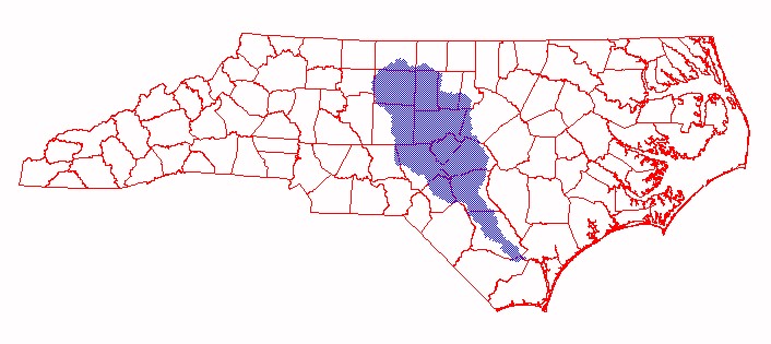
The model is to be used as a primary tool in evaluating current and future water uses of the surface waters as well as enhancing future water resource decision-making in the Cape Fear River Basin. The basin model encompasses approximately 5,255 square miles of land from the headwaters of the Deep, Haw, and Cape Fear Rivers down to U.S. Lock and Dam No.1 which is the limit of tides.
Figure 1-1: Cape Fear River Basin to Lock and Dam #1
Flow conditions in the river vary seasonally as well as annually. The initial goal of the surface water quantity model is for it to be used by municipalities applying for Jordan Lake water supply allocations and inter-basin transfer certifications. Jordan Lake, the largest reservoir within the basin, currently provides water to numerous communities within the basin. All water allocations from Jordan Lake are approved by DWR and are based on the availability of water supply and future water needs.
Since this model is being used as a primary decision-support tool, it was important for the model to be developed in an open, cooperative manner, and to be subject to public scrutiny by all interested parties. The resulting model is a widely accepted and distributed, analytical tool used to develop a consensus among numerous stakeholders within the basin about water resource issues. The model allows users to independently evaluate "what-if" scenarios that provide insight relating to downstream flows. While the model does not include any water quality analysis directly, generated streamflow output can be used in conjunction with most water quality models approved and/or supported by the US Environmental Protection Agency (US EPA).
1.3 Model Selection
The model chosen for the Cape Fear River Basin project is DHI’s MIKE BASIN since it satisfied a majority of the requirements set forth by DWR. The MIKE BASIN engine, which runs within Environmental Systems Research Institute’s (Esri) ArcView environment, allows geographic visualization and query of the model network and components such as withdrawals, discharges, and reservoirs. MIKE BASIN’s capability of running in ArcView affords an opportunity to compile, create, and acquire vast amounts of geographic information that are needed to aid in a basin-wide model. It also provides a convenient geographical interface that makes the model accessible to a broad range of users. The ArcView interface helps define the model, evaluate simulation results, and integrate spatial analysis. Since Geographic Information System (GIS) technology and data is readily available to most governmental entities, potential difficulties are minimized with the use of MIKE BASIN.
In general terms, MIKE BASIN represents the river basin mathematically. It contains the configuration of tributaries and main rivers, hydrology of the basin with respect to space and time, and various water demands. MIKE BASIN incorporates many multisectoral water demands such as domestic water supply, industrial water supply, irrigation, and hydropower generation. It provides a basin-wide representation of water availability, water rights, reservoirs, and transfer/diversion schemes.
2. Data Collection for Model Input and Schematization
The project tasks involved an extensive collection, review, and interpolation of hydrologic data, model schematization, and estimations of agricultural water use as well as municipal and industrial withdrawals and discharges.
The client specifically required that a hydrologic period of at least 65 years be used with a daily time step and that the drought of the early 1930’s be included. The model has been developed for a base case of 69 years with records covering the historical period of 1930 through 1998. This period of record allows numerous sequences of climatic situations ("wet" and "dry") to be analyzed and evaluated.
Data gathering for the Cape Fear River Basin modeling project was an extensive process involving many different parties. This yielded a thorough representation of water resources in the Cape Fear River Basin over the past 69 years, (1930-1998). Government agencies and municipalities as well as private companies have proved to be invaluable data resources in this project and include the following:
An extensive literature review was also performed to help locate additional resources that could be beneficial. Over eighty books and reports were reviewed.
2.1 USGS Gauge Records
To create a 69-year climatic representation of the river basin, naturalized flows were created. These flows represent only the natural flow of the rivers and streams including precipitation and evaporation intrinsically accounted for by the gauge records. Naturalized flows exclude manmade withdrawals and discharges and are the "backbone" of the Cape Fear River Basin model (see Section 3.2). To create these flows, gauge records collected and provided by USGS were used. Currently, 28 gauges are actively recording stream and river flow within the basin. Unfortunately, all of these as well as other recording gauges did not exist for the full 69-year period. Table 2-1 shows the availability of gauge records.
Table 2-1: Availability of USGS Gauge Records
|
Beginning Year |
Number of Gauges |
Currently Recording/Discontinued |
|
1930 |
5 |
Currently Recording |
|
1930 |
14 |
Discontinued |
|
>1930 |
23 |
Currently Recording |
|
>1930 |
33 |
Discontinued |
Twelve gauges were chosen and used to compute the naturalized flow for the model (see Section 3.2).
2.2 NCDC Precipitation and Evaporation Records
Precipitation and evaporation records were needed for input directly into the model for reservoirs as well as to compute agricultural water use (see Section 2.4). NCDC collected and provided all precipitation and evaporation records. Currently, 27 precipitation stations are actively recording. Table 2-2 shows the availability of precipitation data.
Table 2-2: Availability of NCDC Precipitation Records
|
Beginning Year |
Number of Stations |
Currently Recording/Discontinued |
|
1930 |
1 |
Currently Recording |
|
1933 |
5 |
Currently Recording |
|
>1933 |
21 |
Currently Recording |
|
>1933 |
18 |
Discontinued |
Composite county precipitation files were used for agriculture and reservoir input and were created using the Theissen polygon technique described in Section 2.6.
2.3 Municipal and Industrial Withdrawals and Discharges
To obtain 69-years of municipal and industrial withdrawals and discharges, data was received from various state agencies such as Divisions of Water Resources (DWR), Water Quality (DWQ) and Environmental Health (DEH) as well as individual municipalities and industries.
2.3.1 Municipal and Industrial Withdrawals
DWR provided four withdrawal databases: the 1991 and 1993 Water Withdrawal Registration Databases and the 1992 and 1997 Local Water Supply Plan databases. DWR also contacted each withdrawer in the databases by telephone to find out when they began withdrawing water from the Cape Fear River Basin. For industrial withdrawals, DWR requested available hardcopy files. Some municipal withdrawers provided hard copy records.
DEH provided Reports of Plant Operations of monthly withdrawals from each municipal water treatment plant in the Cape Fear River basin from 1990 through 1998.
2.3.2 Municipal and Industrial Discharges
Discharge data was obtained from the NPDES (National Pollutant Discharge Elimination System) permit program regulated by DWQ. The EPA requires each state to establish affluent limitations and performance standards for sources of water pollution, including wastewater treatment plants, industries, power plants, and confined agriculture operations. NPDES records were obtained from 1986 through 1998.
For industrial discharges, DWR requested available hardcopy files. DWR also performed phone interviews for the dischargers to find out when the facility began discharging.
2.3.3 Formulation of 69-Year Time Series
United States Census records were obtained for every 10-year period from 1930 through 1990. Interpolations were performed for existing municipal withdrawal and discharge records, and extrapolations were performed on a per capita basis to synthesize municipal withdrawal and discharge time series for the 69-year period. Where no data existed, industrial withdrawal and discharge time series were computed based on interpolations of existing records and industrial/thermoelectric trends reported in literature. All withdrawal and discharge time series were created as monthly averages to account for seasonal variability.
2.4 Agricultural Water Use
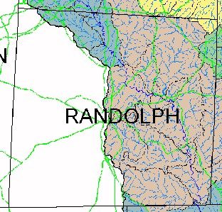
To estimate agriculture water use, multiple variables such as crop acreage, crop demand, livestock counts, and irrigation practices were acquired. County agricultural agents from the NC Cooperative Extension Service, Natural Resource Conservation Service, and Soil Conservation Service were provided with an agriculture questionnaire and were interviewed. During the interviews, agents provided 1998 crop acreages, spatial distributions of crops throughout the county, livestock counts, and surface water irrigation practices for the portion of their county that falls within the Cape Fear River Basin (See Section 2.6 for maps provided to the agents).
Additional agriculture data from NC Agriculture Statistics and from USDA’s Agricultural Census was collected and compiled. NC Agriculture Statistics provided annual reports back to 1990 and intermittently from the 1940’s through the 1980’s. Information in these yearly reports included acreage of tobacco, cotton, soybeans, corn, peanuts, and head counts for livestock in each county. USDA’s Agricultural Census, which is produced on a five-year cycle, dates back prior to 1930. Total and irrigated acreage for tobacco, soybeans, corn, peanuts, and head counts for livestock in each county are contained within the Agriculture Census.
Interpolations/extrapolations were performed with the available data to compute irrigated acreage and livestock headcounts. Dr. Ronald Sneed, former professor from North Carolina State University and former state extension irrigation specialist, advised on the creation of the agriculture questionnaire, "filling in" of data gaps of acreage and headcounts, and water use rates and evapotranspiration curves for the crops and animals.
Data files created for input into the model include irrigated acreage, livestock totals, livestock demands, crop demand curves, and whether the irrigation equipment are moveable or fixed systems. See Section 3.4 for agriculture dialog box.
2.5 Reservoirs
NC Dam Safety Database was obtained to get a complete listing of reservoirs within the basin. This database contains over 4800 dams throughout NC with over 80 field entries per dam. National Dam Safety Program Inspection Reports were also provided by NC Dam Safety. These inspections were performed by the Army Corps of Engineers in the 1980’s. These reports yielded the following information:
To further enhance the information gathered, numerous municipalities and design engineers were contacted about their water supply dams, and field reconnaissances were performed. Additional information about minimum releases, stage-storage relationships, and operating procedures was acquired from the telephone interviews.
For specific information on Jordan Lake, the Wilmington District of USACE provided area/capacity curves, the water control plan, and elevation/inflow/outflow files.
Dams/reservoirs not used for water supply purposes were not included within the model.
2.6 Geographic Information
2.6.1 Geographic Information System (GIS) Coverages
All GIS coverages were provided by either NC Center for Geographic Information and Analysis through DWR or created from ASCII files. These coverages aided in:
Figure 2-1: Sample Map Used During Agriculture Extension Agent Interviews
GIS coverages were created for all data that had an associated latitude and longitude. Created coverages include:
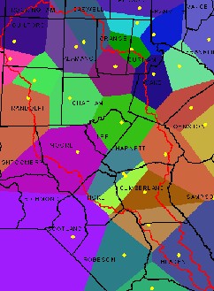
The creation of these coverages gave a spatial reference to dams, withdrawals, and discharges so that they were input into the model in their correct location. The streamflow gauge coverage aided in visualizing the distribution of gauges throughout the basin. The precipitation coverage aided in visualizing the distribution of stations throughout the basin (see Figure 2-2). Theissen Polygons were created around the precipitation stations using ArcView Spatial Analyst, and composite county precipitation files were created (see Figure 2-3).
Figure 2-2: Spatial Distribution of Precipitation Stations

Figure 2-3: Theissen Polygons of Precipitation Stations
2.6.2 Digital Elevation Model (DEM)
A 60-meter DEM was acquired from the North Carolina section of USGS for use in the model. A DEM can be defined as a sample array of elevations for a number of ground positions at regularly spaced intervals. DEMs are produced from either map contour overlays that have been digitized or from scanned aerial photography. The DEM was used for delineating catchments and creating the river network in the model (see Section 3.1).
2.7 Committee Review of Input Data
Throughout the project term, the data collection and modeling efforts were reviewed extensively and methodically by a technical review committee composed of representatives from local governments and state agencies established by DWR for the Cape Fear River Basin project. Input data and methodology statements were provided to the technical review committee and stakeholders via M&N’s File Transfer Protocol (FTP) site. Numerous consultant and committee meetings were held to get group input and feedback. Comments were received, reviewed, and formally addressed; the final dataset reflects changes made due to technical review committee comments.
3. Model Construction
The Cape Fear River Basin model provides a comprehensive representation of the river basin. The river system is represented to the degree necessary to depict all important features. It includes all significant discharge/withdrawal points (see Section 3.5), irrigation demands distributed within each county, and major reservoirs. Long time series covering the period from 1930 through 1998 have been developed in order to include sequences of "dry" and "wet" climatic events. The model has been developed so that either daily or monthly time steps can be applied.
3.1 Modeling Features
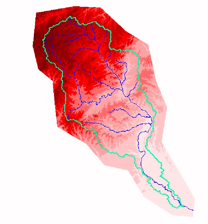
The Cape Fear River system presented in the model was developed from a 60-meter Digital Elevation Model (DEM) provided by the North Carolina section of USGS. The Cape River system is highly detailed and complex. In the model only the main river and tributaries, which are important to represent major points of interest such as significant withdrawals or discharges were included (see Figure 3-1).
Figure 3-1: Clipped DEM for the Cape Fear River Basin
River nodes have been included to represent:
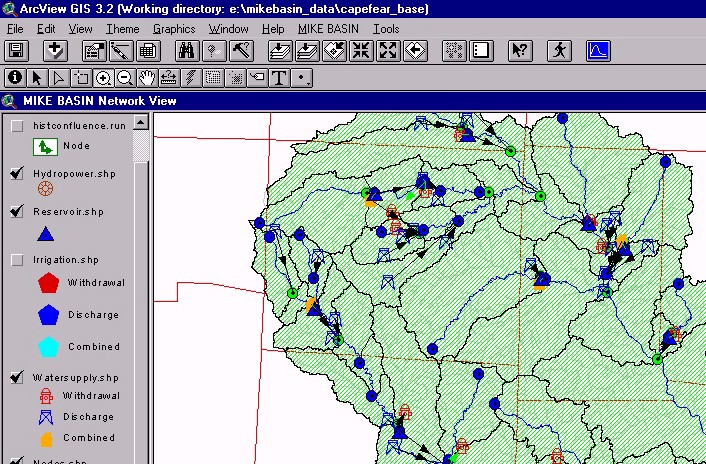
Figure 3-2 shows a small a part of the model area. It illustrates the detail of the river system and the sub-watershed delineation. The blue river sections are the river sections represented in the model. The picture also shows the location of nodes and withdrawal/discharge points.
Figure 3-2: Detailed View if the Generated Sub-basins Showing Nodes, River Network, and Sub-basins Represented in the Model
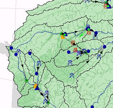
In the model, catchment nodes have an up-stream sub-watershed attached with a respective unit runoff. Intermediate nodes have no sub-watershed attached but have withdrawals, discharges, or reservoirs attached. The model area is divided into 73 sub-basins. A total of 119 nodes were included at which flow is computed. Fourteen of these nodes are represented as reservoirs, 102 are represented as discharge/withdrawal nodes, and 43 are represented as irrigation demands.
Available GIS coverages were used extensively and provided critical information during the model development (see Section 2.6). The GIS data distributed with the model includes coverages of sink/sources, county boundaries, reservoir locations and location of gauging stations.
3.2 Estimation of Unit Runoff
Unit runoff is defined as the quantity of water per unit area that enters the river from a well-defined watershed. The naturalized flow (see Section 2.1) is the instream flow at a given location in the river that would have occurred without the influence of man's activity.
The unit runoff was not known, but had to be estimated. The methodology used in model was to determine naturalized flow at given locations in the river system where gauged flow data exist. From the naturalized flow, the unit runoff was calculated as the flow augmentation between two gauging stations divided by the watershed area.
The general equation for calculation naturalized flow is:
NF = GF + W - D + RA - RF
Where NF is the naturalized flow; GF is the gaged flow; W is withdrawal; D is discharge; RA is reservoir adjustment; and RF is return flow. The naturalized flow was estimated based on the gauged flow and by reconciling (using addition, subtraction, and lag) all known deviations from the natural conditions. Deviations from natural conditions include diversions, withdrawals, discharges, influence of reservoirs, and other operations in the river system.
At a given location, the procedure used to determine unit runoff in the model was to match the simulated and gauged streamflow using an apriori unit runoff time series as a first estimate. By recording the deviation at every time step the unit runoff was modified until an acceptable match was obtained between the observed and simulated flow. Under certain ideal conditions a nearly perfect (100 %) match could be obtained with the monthly time series. However, because of routing conditions and possible inconsistencies in the gauged data, as well as withdrawal/discharge data, a perfect match could not be expected with the daily time series.
The model was divided into 12 runoff areas having homogeneous runoff patterns (see Figure 3-3) delineated from the 12 selected gauging stations. These 12 gauging stations provided long-term historical flow records. In some cases, the station records for the individual stations did not cover the entire period. Records were, in such cases, completed by station to station transposition with the nearest representative station.
Figure 3-3: Distribution of Runoff Areas Having Homogeneous Unit Runoff Pattern
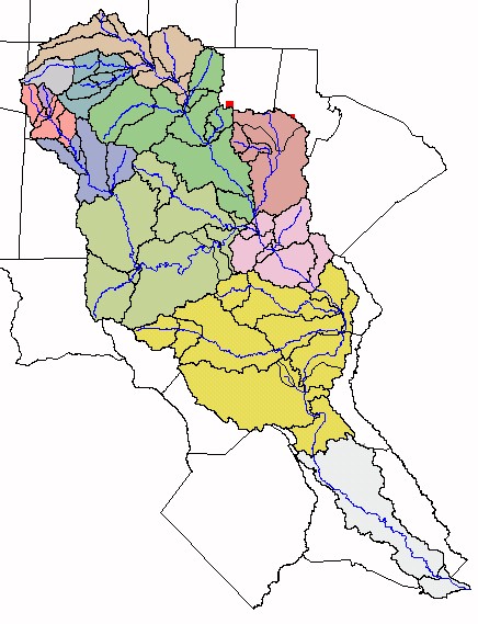
For each comparison with gauged data, the procedure was to run a sub-model covering the model area upstream of the gauging station. If another gauging station used for calibration was located upstream of the station, only the watershed area between the two stations was considered for that particular estimation, and the upstream gauging station was used as the upstream boundary. In this way, the errors in upstream estimates were not accumulated in the downstream direction.
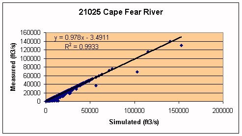
The estimations showed in all cases very close matches between observed and simulated hydrographs, which was not surprising considering that the naturalized flow was estimated on the basis of the gauged data. However, uncertainties in routing parameters, reservoir operations, and inconsistencies in gauging data contributed to a less than 100% perfect match in some cases. Representative statistics are shown in Figures 3-4 through 3-6. Note the square of the Pearson product moment correlation coefficient, R2, was computed for the x and y data points for various locations. The r-squared value can be interpreted as the proportion of the variance in y attributable to the variance in x. For a perfect model, R2 = 1.0.
Figure 3-4: Gauge Station 02102000, Deep River at Moncure
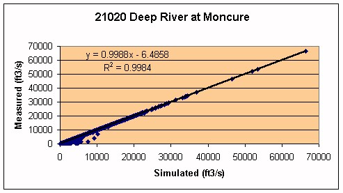
Figure 3-5: Gauge Station 02096960, Haw River at Bynam
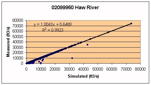
Figure 3-6: Gauge Station 02105769, Cape Fear River at Lillington
3.3 Reservoirs
The model accommodates two types of reservoirs:
A Standard reservoir is regarded as one physical storage, and all users are drawing water from the same storage pool. If there are several users drawing water from the reservoir a priority is attached to each user. A set of operation rules applies for each user to draw water from the storage.
The Allocation Pool reservoir is also simulated as one physical storage, but the volume in the reservoir is sub-divided based on different uses such as flood control, water quality (low flow augmentation), water supply, and sedimentation storage. In the present case, individual users were allocated a certain percentage of the total water supply storage pool. This was the primary issue for Jordan Lake. In the Jordan Lake scenario, the model incorporates an accounting procedure that tracks the actual water storage in one pool for downstream minimum flow releases (water quality pool) and in the six other pools allocated for water supply users. Inflows and rainfall to the reservoir are distributed among various storage accounts and evaporation losses are likewise spread among the users. For each pool a set of operation rules applies.
Fourteen reservoirs are represented in the model. Each reservoir is described by its reservoir characteristics:
To complete the water balance computations for a reservoir, time series files for direct rainfall and evaporation to and from the water surface were specified. Composite county rainfall and evaporation files were used (see Section 2.6). The operating rules for each reservoir was specified. These rules describe basic reservoir characteristics (e.g. full reservoir level) and various water levels at which certain operation rules take place (e.g. flood control level, normal operating zone, reduced operating zone, and conservation zone). Sets of reduction factors were specified for each down-stream user. Reduction factors specify a portion of demand that is fulfilled if the reservoir level falls into the reduced operating zone specified in the operating rules. These reduction factors are used during the simulation depending on the related reduction zones or levels specified in the operating rules. For the Standard Reservoir option, two reduction factors and respective reduction levels were specified, and for the Allocation Pool option, four reduction factors and respective reduction levels were specified. Default values are given in the dialog when the number of users has been specified.
3.4 Agriculture Demands
The agricultural water usage was calculated for the period 1930 through 1998 for each county in the river basin area. The total usage was distributed as withdrawals in different parts of the river system according to its assumed distribution within each county (see Section 2.4). Irrigation demands for the 17 counties within the river basin were divided into 43 time series and were used as withdrawals in the model. See Section 3.6 for project specific code development details for agriculture.
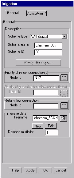
As part of the project requirement, a dialog (see Figure 3-4) was developed in the model to calculate irrigation demand time series directly in the model. The agricultural demand time series can be calculated based on information about cropping patterns and acreage, livestock demands and populations, as well as rainfall. Agricultural demands are calculated from crop and livestock information when the Agriculture input field is enabled in the Agricultural tab of the Irrigation dialog.
Figure 3-4: Agriculture Input Dialog Box
Crop demand curves are time series of the water demand for each crop included in the withdrawal point. The time series can be given with any time resolution and there are no limitations on the number of crops to be included. If crop demand curves are given for one year, the curves can be used for other years in the simulation period.
For some of the crops, moveable machinery is used for irrigation, and these crops may be watered only occasionally. In such cases, adjustments for rainfall are accounted for in the irrigation scheduling. For other crops, a fixed irrigation schedule may be applied without considering rainfall.
Adjustment for rainfall is carried out for each time step by comparing the rainfall with the crop water demand:
If C> R: I = C – R
If C< R: I = 0
Where C is crop water demand (e.g. in/day), R is rainfall (in/day) and I is irrigation (in/day).
Livestock demand curves are time series of the water demand for each animal included in the withdrawal point. These time series can be given with any time resolution and there is no limitation on the number of different animals to be included.
Historical rainfall data for the period 1933-98 were used in order to account for variations in climate. Agricultural withdrawals from 1930 to 1933 were assumed to be equal to the demands of 1933, since no rainfall data existed prior to 1933. Some agricultural demands are constant demands, however, others such as tobacco demands are based on rainfall. Rainfall-related agricultural water demand time series were constructed by examining seven-day time intervals. Rainfall was summed for one week, and agricultural demand was summed for one week. Where shortfalls in rainfall occurred, irrigation was assumed to make up the difference. This amount of irrigation was assumed to be evenly distributed over the following week but was not taken into account as part of the rainfall totals of that particular week. By computing these series on a seven-day basis, the root zone storage is allowed to accumulate rainfall.
3.5 Withdrawal and Discharge Water Usage
The Cape Fear River Basin model includes:
The combined option was used wherever unique relationships appeared between the withdrawal and discharge; the discharge was never higher than the withdrawal at any time in the records.
3.6 Project Specific Code Developments
While the existing version of MIKE BASIN was quite broad and adaptable, none the less, certain requirements were needed at the source code level to adequately represent the needs of the project.
3.6.1 Jordan Lake Reservoir
The most significant dedicated feature is the Allocation Pool option for reservoirs which includes a release policy according to downstream flow targets (see Section 3.3).
For each time step (e.g. each day) in the simulation, the allocation pool is simulated as follows:
1. Inflow from the upstream river(s) is added to the reservoir main storage.
2. The reservoir level and the surface area are calculated based on the reservoir area-capacity curves.
3. Precipitation, based on the actual reservoir surface area is added to the reservoir main storage.
4. Evaporation losses, based on the actual reservoir surface area and weather conditions, are extracted from the reservoir main storage.
5. Bottom infiltration, based on the actual reservoir surface area and a user-defined infiltration velocity, is extracted from the reservoir main storage.
6. The individual water supply pools and the water quality pool are updated by adding a user-defined fraction of total reservoir net-inflow to these pools. If the sum of evaporation losses and bottom infiltration is greater than the sum of upstream river inflow and precipitation, this reduces the water volume of these pools. If the contribution is greater than the remaining capacity of the individual pool, water spills to a common storage.
7. If there is any water in the common allocation storage, this is distributed to water supply pools and the water quality pool in case these are not already filled using the same distribution key as for the reservoir inflow. If all pools are filled during this procedure, the reservoir level is at or above the guide curve. This means that some water is available for common use. The common storage is used to fulfill water quality releases, then any remaining water is used to fulfill demands from water supply nodes connected to the reservoir.
8. In order to meet the minimum downstream release requirements (water quality release), water is subtracted first from the common storage if possible, then (if needed) from the water quality storage. If a downstream control node is defined, MIKE BASIN tries to meet the user specified minimum target flow for this node by taking into account inflow from the Deep River and runoff from the intermediate watershed area.
9. For each individual user, in order of priority, the model tries to fulfill the individual water demand. First, water is extracted from the common storage if possible, then (if needed) from the associated water supply pool. Extraction from the water supply pool may be reduced due to user specified reduction volume thresholds and associated reduction factors (see Section 3.3).
10. If the reservoir water level, after releasing water to ensure minimum release and distributing water to the reservoir users, is still above the flood control level, water is released to the downstream river in order to lower the reservoir level to the flood control level. The total release rate from the reservoir does not exceed the user-specified maximum downstream release rate (normally equal to the maximum non-damaging release rate). Furthermore, if a downstream control node is defined, the model attempts to regulate the release in order to keep the river flow rate at the control node under the user defined maximum flow rate.
If the reservoir level still is above the reservoir full level, additional water is released in order to lower the level to the reservoir full level (disaster situation). In extreme situations the releases may be at the maximum rate that can be conveyed by the reservoir outlet works and spillway without consideration of downstream stages..
3.6.2 Low Flow Statistics
The following low flow statistics are calculated for flows at each river node:
The low flow statistics are calculated from moving average figures and subsequently ranked from the smallest to the largest yearly values and subjected to frequency analysis using the Log-Pearson Type III distribution. They are provided in a monthly output table.
3.6.3 Multipliers in Dialogs for Water Supply and Agriculture Demand Time Series
A demand multiplier was included in the water supply and agriculture dialogs. Use of multipliers is a convenient way of modifying the demand input for sensitivity analyses.
3.6.4 River Routing
Routing is important to take into account when there is a significant delay and smoothing of the flow hydrograph between two river nodes. This is often the case if the distance between two nodes is large or the model is run with small time steps e.g. daily time steps.
The routing method adopted is the Muskinghum method, which is a commonly used hydrologic routing method for handling a variable discharge-storage relationship. This method models the storage volume of flooding in a river channel by a combination of wedge and prism storage. During the advance of a flood wave, inflow exceeds outflow, producing a wedge of storage. During the recession, outflow exceeds inflow, resulting in a negative wedge. In addition, there is a prism of storage, which is formed by a volume of constant cross section along the length of the prismatic channel.
3.7 User Scenario Modeling
Based on the above model setup and code modifications the user is able to run the model on a daily time step for the full 69-year period of record, and thus able to analyze various what-if scenarios for changes made as a result of the following:
Impacts of the above changes can be analyzed at each node (including reservoirs) based on summary tables and graphs generated by MIKE BASIN. The user is thus able to make decisions regarding water supply issues along the entire basin.
4. Documentation, Training, and Software Support
Project requirements specified that detailed documentation, user manuals, training, and software support be provided with the Cape Fear River Basin Model.
A detailed document describing the data set preparation and model formulation was provided with each licensed model copy. Also, a MIKE BASIN User’s Manual with a tutorial adequate for use by less technical staff was provided.
Initially, model training was provided to DWR and other local government staff and their consultants. Participants learned how to (1) evaluate impacts of the Jordan Lake allocations applications and associated interbasin transfer (IBT) requests, and (2) perform drought management planning and forecasting. At project completion, the model was widely distributed (20 installations), and therefore, required more extensive training. All interested stakeholders attended either a general or an in-depth training session.
Remote software support will be provided for up to five years following model delivery.
5. Conclusion
The Cape Fear River Basin Model has proved to be a successful GIS-based tool for evaluating current and future water uses of surface waters in the Cape Fear River Basin (see Figure 5-1). Since the model was developed in an open, cooperative manner, it has been widely accepted and distributed. The model currently allows stakeholders to independently evaluate "what-if" scenarios that provide useful analyses concerning water resource issues. Stakeholders are able to evaluate impacts of the Jordan Lake allocations applications and associated interbasin transfer (IBT) requests and perform drought management planning and forecasting. Currently, the model allows water quantity modeling, but with little effort can be extended to incorporate water quality.
Figure 5-1: Cape Fear River Basin Model
Sheila Thomas Ambat
Jesper Kjelds