Rick Hanson
The Truth About Airborne GPS
Though airborne GPS has been widely used since1993, there is still a wide
diversity of opinions as to how much ground control is required and where the
control should be placed. In the spring of 1999, Merrick & Company entered
into a contract with the County of Boulder, Colorado to provide aerial
photography and digital orthophotography of the eastern two-thirds of the
county. The project would be controlled by airborne assisted analytical
aerotriangulation with approximately 65 widely dispersed, targeted control
points. This paper examines and compares the results of five sets of aerial
triangulation data generated from various control configurations.
INTRODUCTION
Background
Because of the expense of field control for a
photogrammetric mapping project, photogrammetrists have always been interested
in ways to reduce the amount of field work involved with producing a reliable
product. Conventional control methods required no less than 4 field points for
each stereo model. When analytical aerial triangulation (AT) came into wide use
in the late ‘60’s the number of required field points was reduced to
approximately 1 point for every 3 stereo models. With recent advancements in GPS
technology an entire project can be controlled by as few as three field points.
Some even say that zero control points are required, but a photogrammetrist will
always want some way of performing a qualitative check of his or her work in
order to guarantee the accuracy of the final product. This means that sooner or
later some field measurements will be required so they might as well be done in
advance of the aerial triangulation. The uncertainty comes with deciding how
many control points to use, and where they should be placed.
Overview
Since the Boulder County scope called for 65 control
points, approximately 1 point for every 2 stereo models, the photogrammetrists
at Merrick took advantage of the situation by performing a number of adjustments
using various control configurations holding only five points for the AT
adjustment and using the remaining 60 points for checks.
Aerial Photography
The project located near the eastern foothills of
the Rocky Mountains covers an area of 400 square miles. Black and white aerial
photography was flown at a height of 12,000 feet above mean terrain with 60%
endlap and 15% sidelap. A GPS receiver in the aircraft collected satellite data
at 1 second intervals along with an event mark generated by electronic impulse
each time the camera exposed a photograph. A GPS ground station was positioned
at Jefferson County Airport, ten to fifteen miles from the project area. Seven
north-south flight lines covered the project area with a total of 160 exposures.
All of the photography was flown on the same day under optimum conditions using
a Wild RC-30 precision mapping camera with forward motion compensation (FMC).
Field Control Merrick measured 65 pre-targeted points by post-process kinematic
method using two base stations and collecting satellite data at 3 second
intervals for a minimum of 15 seconds so that no less than 3 epochs were
recorded for each station. The expected accuracy for this exercise was +/- 0.1’
horizontally and +/- 0.5’ vertically, accuracy’s more than adequate for the
production of 1”=400’ digital orthophotos to an accuracy of +/-3.4 feet for 90%
of the points measured. Aerotriangulation Aerial photographs were pugged with 3
pass points in each photo and flight lines were joined with 1 tie point for each
adjacent photograph. Then control targets and analytical points were measured on
Zeiss P1 analytical stereo plotters. Measurements were processed using
Eriotech’s ALBANY software. With due consideration for aircraft GPS antenna
offset and exposure impulse time delay, post processed airborne GPS data was
combined with field control, flight and camera calibration data to produce final
AT coordinates.
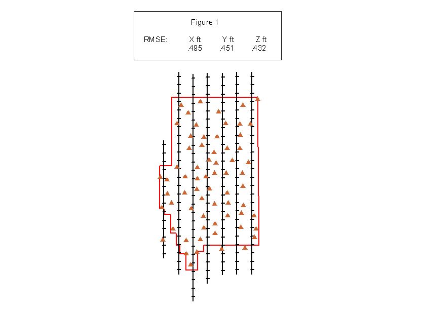
The first adjustment was performed holding all 65 field
points as control. Results of the first adjustment are shown in figure 1.
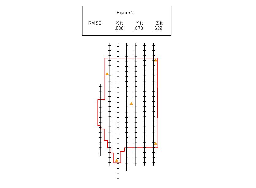
A second adjustment was performed by holding 5 field points, 1 near each corner of the
project and 1 near the center of the project area. The remaining 60 points were
used as check points only. This is seems to be the preferred configuration of
control for an airborne GPS project. The RMSE’s of the check points in the
second adjustments are shown in figure 2.
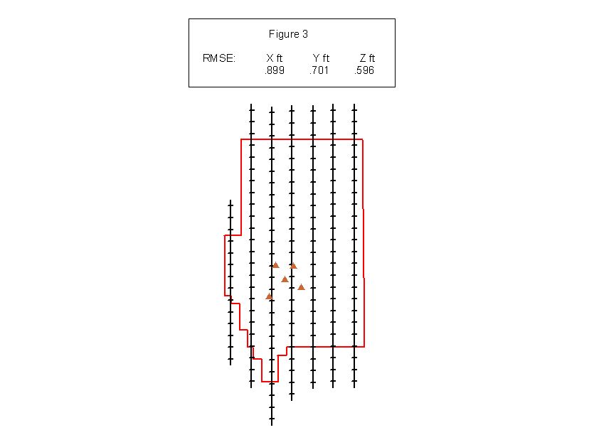
At first glance, the control placement for
the next three scenarios would appear to be insufficient to support accurate
aerial triangulation but the results indicate otherwise. The third AT adjustment
shows the RMSE’s of the 60 check points as controlled by 5 points closely
grouped near the center of the project area. Result of the third adjustment are
shown in figure 3.
The fourth adjustment shows the RMSE’s of the 60 check points controlled by 5 points
aligned in a north-south direction ranging the length of the project area.
Results of the fourth adjustment are shown in figure 4. 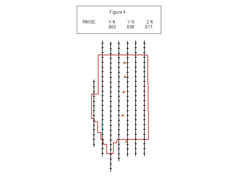
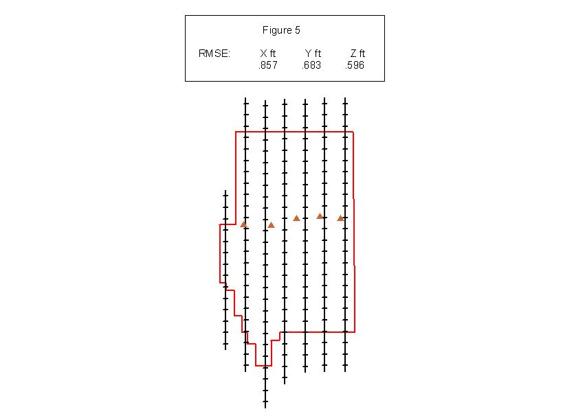
The fifth AT adjustment, shown in figure 5,
shows the RMSE’s of the 60 check points as controlled by 5 points arranged in an
east-west direction ranging the width of the project area.
Summary of results
|
Xft |
Yft |
Z ft. |
| Adjustment 1 RMSE: |
.495 |
.541 |
.432 |
| Adjustment 2 RMSE: |
.838 |
.678 |
.629 |
| Adjustment 3 RMSE: |
.899 |
.701 |
.596 |
| Adjustment 4 RMSE: |
.880 |
.696 |
.617 |
| Adjustment 5 RMSE: |
.857 |
.683 |
.596 |
CONCLUSION
Though the first aerial triangulation adjustment using all of the
points as control yields the best results, it is not practical to develop 1
field control point for every two stereo models as the abundance of control
obviates the need for airborne GPS. The RMSE’s of scenarios 2,3,4 and 5 show
more than sufficient accuracy’s on the check points to support 1”=200’ mapping
with a 5’ contour interval, more than twice as accurate as Boulder County’s
project scope called for. If we accept that only five field points are required
to control a given block of photography, and this does appear to be the case,
the question of control placement seems to be answered by the negligible
differences in the results of adjustments 2,3,4 and 5. When significant figures
are taken into account, the placement of the field control matters very little
in a practical production environment.
As to the question of the number of
control points that should be used in a given project, every project is
different and often the number of points is controlled by what the budget will
bear. Additionally, if we think of the check points as confidence points the
number may vary according to the confidence level of the photogrammetrist to
produce accurate data over a given area at a given altitude. When all else
fails, the author suggests not less than 10% of the number of exposures it takes
to cover the project area at the prescribed photo scale, using as many of the
points a possible for check points.
Acknowledgments
I must thank Paul Tessar, Boulder Counties GIS
Director, for permitting me to use his project as a topic for my paper.
Aero-graphics, Inc. of Salt Lake City did a very professional job of the aerial
photography and airborne GPS data collection and post processing. Brian Raber of
Merrick & Company in Aurora, Colorado for encouraging me to write this
paper.
Rick Hanson
Project Manager and Certified Photogrammetrist
Merrick
& Company, Aurora, Colorado