 (2)
(2) The University of Texas-El Paso developed a GIS for Texas DOT to automate the routing of super-heavy vehicles. The GIS uses a network representation of the highways with attributes linking to a bridge information database. Given vehicle characteristics and points of origin and destiny, shortest paths and bridges along routes are found. Information is retrieved from the database and bridge adequacy is evaluated from established formulae. Network segments containing inadequate bridges are disabled and new paths are searched repeating the process until a suitable route is found. Information management issues are addressed that may benefit the transportation community.
The Motor Carrier Division (MCD) of the Texas Department of Transportation (TxDOT) is the agency that issues permits for overweight and oversize vehicles traveling through the state highways (see Figure 1). These are referred to as the On-system highways. With the continuing increase in commerce and trade in Texas, the MCD continues to experience increases in the number of permits issued for these types of vehicles. Some of the permit requests are for super-heavy loads, that is vehicles in excess of 300,000 pounds up to one million pounds.
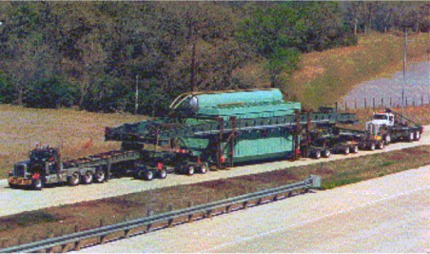
Figure 1. Typical super-heavy vehicle (Courtesy of MCD, TxDOT).
The customary procedure for processing these requests is time consuming and costly. The process consists of:
a) manually establishing a tentative route,
b) identifying all the bridges on the route,
c) obtaining the information of the bridges to be crossed;
d) analyzing for the structural adequacy of the bridge for the super-heavy vehicle.
Alternate routes are investigated, as some bridge structures are found inadequate. As an effort of reducing the time to process the permits, it is becoming customary to re-use portions of routes already analyzed for greater loads. This approach may cause future infrastructure problems due to repeated overloads.
The current permitting procedure followed by MCD is based on the rules and regulations for movement of oversize/overweight loads governed by the Texas Administrative Code [1] (TAC).
These regulations limit the loads based on a gross axle weight criterion (which depends on the number of axles per axle group) and a tire pressure criteria of 650 pounds per inch of tire width, except for special vehicles such as mobile cranes where the pressure criteria is 850 pounds per inch.
If either criterion is exceeded, TxDOT's Design Division performs an analysis of the bridges along the vehicle's route to determine if a permit may still be issued. The significant drawback of analyzing each bridge is that the engineering efforts are time consuming and costly.
TxDOT sponsored research aimed at developing guidelines for effective general procedures for issuing permits for super-heavy vehicles passing through Texas. Two different types of formulae were developed for bridges exceeding or reduced to designations other than H15, H20, HS-15 and HS-20 (i.e. HX or HSX):
1) a general formula, not dependant on the bridge span length, and
2) a bridge-specific formula that accounts for the bridge span length.
The bridge load formulae (BLF)developed at TTI [2] were found suitable for implementation in an automated route evaluation system.
This paper describes the development of an operational Geographic Information System (GIS) to route super-heavy and oversize vehicles on the Texas highways using ArcView software.
To develop the proposed GIS a series of requirements were defined and a thorough survey was performed to identify the available information.
Required basic components:
1) A highway network model representing the On-system roads, developed from digitized maps containing at least a classification of highways, e.g. Interstate highways, State highways, Farm to Market roads, etc. and their corresponding designations. Other desired features include directions of travel and road mileage preferably in database format;
2) A bridge network coverage with a access to a comprehensive series of attributes such as bridge identification, number of spans, span lengths, design ratings;
3) A route evaluation model to handle heavy-loads and
3) GIS software suitable for transportation modeling.
Selected resources identified during the survey:
1) Use TxDOTs official digitized County/Urban maps available from the Mapping Office of the Transportation Planning and Programming Division (TPP) in Intergraph's DGN format. The primary reason for selecting these drawings was the completeness and comprehensive amount of details, containing the geometric characteristics of overpasses, underpasses, interchanges and exit ramps, needed to perform a comprehensive routing through the On-system roads. The geographic features are classified and organized in 64 layers. One of the layers contains the symbols representing the location of bridges. A limited database containing a few highway names was available and was linked to the maps.
2) Use TxDOT's Bride Inventory Inspection and Appraisal Program (BRINSAP) database. BRINSAP was the only bridge database available with sufficient bridge geometry data, including the geographic locations in world coordinates format. The database is available in MS Access format.
3) Use ArcView GIS software to develop the routing application.
3) Implement within the routing model, both the rules adopted by MCD and the developed bridge formulae to determine the feasibility of issuing a permit for heavy/overdimensional vehicles.
Two critical elements for the success of the routing GIS were:
a) to account for all bridges along a given route, and
b) to have an accurate road network model that includes traffic flow directions.
The GIS routing application mainly requires two coverages. One consists of a line coverage with the On-system roads and a point coverage representing the bridge locations. Additional, non-required line coverages may be created for spatial reference of the roads and bridges. These include a bridge symbols coverage and a city streets coverage.
All line coverages were created, exporting the corresponding layers in the TxDOT County/Urban file drawings and converting them into the GIS coverages. The bridge locations were mapped into a point GIS coverage using the longitude and latitude coordinates of the bridges stored in BRINSAP.
After superimposing all coverages, several problems were identified. The bridge coverage showed several bridge location problems, including incorrect/offset bridge coordinates or missing coordinates (see Figure 2). The database was further explored for completeness of information and as a result, occasional missing attributes (e.g. span lengths, ratings, etc.) were observed for some records.
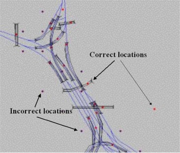
Figure 2. Problems with bridge coordinates.
On the other hand, the roads coverage required significant amount of processing to convert it into a network model. Typical problems encountered include: duplicate line segments, undershoots, overshoots, crossover without connection and disconnectivity (see Figure 3). Moreover, the only attributes available include the highway names, which are only attributed to the centerlines of divided highways, and travel directions were not available.
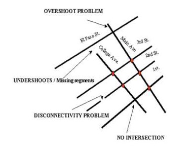
Figure 3. Problems with road network connectivity.
Other occasional problems include missing bridge symbols and geographic features allocated in different layers with respect to their corresponding ones.
Corrective measures were conducted to prepare the road network for routing. The corrections were accomplished by re-importing all previously mentioned geographic features from the County/Urban files into a third party GIS software.
The corrective measures include:
The locations were verified using database information in BRINSAP and printed maps.
The bridge locations were corrected by editing the points to its correct location.
Eliminate repeated line segments, fix overshoots and undershoots
Assign highway names and directions of travel to divided highways, one-way roads, interchanges and exit ramps.
Define
overpasses/underpass at intersections.
Assign bridge structure number to corresponding road segments to automatically identify bridges as functions of vehicle routes.
The road network preprocessing was accomplished using previously developed custom-made macros that semi-automated the editing tasks. During the preprocessing phase, the database structures of the GIS coverages were slightly altered to accommodate for compatibility with the software.
The GIS conversion process as well as the corrective strategies is described in detail in reference [3] since it is beyond the scope of this paper.
As stated earlier, the MCD verifies that the maximum legal weights are met, to determine the feasibility of issuing a travel permit for a given vehicle. The disadvantage of this criteria is that it only considers the vehicle axle loads and configuration, ignoring bridge geometry and type.
To avoid the excessively long waiting periods and expensive structural analyses of all the bridges along a proposed route, a set of bridge load formulae were developed.
In general, the criteria to determine a routes adequacy is as follows:
BRINSAP includes several fields where bridge data is collected, stored and updated periodically.
Some of the bridge information includes:
۶ Bridge structure numbers as identifiers
۶ Minimum underneath vertical clearance
۶ Total horizontal clearance (over and underneath)
۶ Number of bridge spans
۶ Total bridge length
۶ Length of largest span
۶ Bridge type (simple or continuous)
۶ HX or HSX operating rating
Considering the available bridge information, and that the information can be retrieved from BRINSAP, since bridges can be identified as a function of traveled routes through the bridge structure identification numbers (SN) attributed to the road segments of the network, the aforementioned route adequacy evaluation process can easily be implemented in the proposed automated routing system.
The Texas Rules and Regulations under the TAC specify various limits in vehicle size and weight for movement of oversize/overweight vehicles. The following is a summary of the axle group weight limits allowed for issuing permits that are in excess of the maximum legal weights.
Table
1. TAC Axle Group Weight Restrictions
|
of Axles per Group |
Maximum Allowable Axle Group Weight (Kips) |
Maximum Distance Between Extremes of any Group of Two or More Axles (Feet) |
Maximum Legal Loads (Kips) |
|
1 |
25.0 |
- |
20 |
|
2 |
45.0 |
10 |
34 |
|
3 |
60.0 |
32 |
42 |
|
4 |
70.0 |
51 |
50 |
|
5 |
81.4 |
51 |
58 |
The bridge load formulae developed by Keating et al [2] determines the maximum allowable loads for the axles groups associated with a given vehicle. A brief overview of the formulation follows.
The maximum allowable axle group weight as defined by Equation (1) is corrected by incorporating reduction factors that account for gage distance and number of tires per axle. Equation (3) defines a general formula to limit the weight of any group of axles by the bridge design type and the group wheelbase; while equation (4) defines a bridge-specific formula that in addition to the above factors also accounts for the span length of the bridge.
 (1)
(1)
where:
GWrev = Revised axle group weight, kN (kips);
Si = reduction factor for each axle with more than four tires per axle;
1.0 for axles with four tires or fewer;
0.96 for axles with eight or more tires;
n = number of axles;
Ri = reduction factor accounting for gages wider than 1.8 m (6 ft.) calculated by the following formula;
 (2)
(2)
GW = axle group weight, kN (k), calculated from either equations (3) or (4 and 5):
GW = ( a + b WBrev) X (3)
GW = w * WBrev (4)
 (5)
(5)
where:
w = allowable distributed load, kN/m (k/ft.);
L = span length, m (ft.);
WBL = WBrev , m (ft.) when WB < L;
L, m (ft.) when WB >= L;
X = design rating of the bridge;
a,b,c,d = regression constants (see Tables 2 and 3 or Osegueda et al 1999)
[4];
WBrev = revised wheelbase, m (ft.);
The revised wheelbase is defined in equation (6) as:
 (6)
(6)
where:
WB = vehicle wheelbase, m (ft.);
b = correction factor for concentrated loadings;
1.0 for continuous span bridges;
defined for simple span bridges as the lesser of Equations (7 or 8):
 (7)
(7)
 (8)
(8)
where:
D = distance between the center of gravity and nearest axle, m (ft.);
GD = greatest distance between any of two axles, m (ft.).
Table
2. Constants for General Formula
|
Bridge
type |
Impact |
a |
b |
|
|
0% |
17.83 - 0.034X |
1.973 -
0.0119X |
|
|
|
(4.009 - 0.0077X) |
(0.1265 -
0.0012X) |
|
HX |
10% |
16.21 - 0.031X |
1.804 -
0.0172X |
|
|
|
(3.645 -
0.007X) |
(0.1157 -
0.0011X) |
|
|
30% |
12.81 - 0.027X |
1.684 - 0.016X |
|
|
|
(2.88 -
0.006X) |
(0.108 -
0.001X) |
|
HSX |
0% |
0.0 |
3.103 - 0.016X |
|
|
|
0.0 |
(0.199 -
0.001X) |
|
WB < 11.6 m |
10% |
14.45 +
0.0013X |
2.791 - 0.013X |
|
(WB < 38
ft.) |
|
(3.249 +
0.0003X) |
(0.179 -
0.0008X) |
|
|
30% |
13.08 -
0.0623X |
2.136 +
0.0062X |
|
|
|
(2.94 -
0.014X) |
(0.137 +
0.0004X) |
|
HSX |
0% |
35.52 -
0.0342X |
1.380 - 0.016X |
|
|
|
(7.985 -
0.0077X) |
(0.0885 -
0.001X) |
|
WB < 11.6 m |
10% |
32.27 -
0.0756X |
1.258 - 0.014X |
|
(WB < 38
ft.) |
|
(7.255 -
0.017X) |
(0.0807 -
0.0009X) |
|
|
30% |
24.64 +
0.0356X |
1.325 - 0.016X |
|
|
|
(5.54 +
0.008X) |
(0.085 -
0.001X) |
Table
3. Constants for Bridge-Specific Formula
|
Bridge
Type |
Impact |
a |
b |
c |
d |
|
|
0% |
2.262 - 0.0204X |
0.0 |
459.1 - 1.376X |
225.5 + 0.994X |
|
|
|
(0.155 - 0.0014X) |
0.0 |
(-1111 - 3.33X) |
(166.3 + 0.733X) |
|
HX |
10% |
2.320 - 0.0350X |
0.0 |
442.5 + 0.4835X |
202.7 - 0.949X |
|
|
|
(0.159 - 0.0024X) |
0.0 |
(-1071 + 1.17X) |
(149.5 + 0.7X) |
|
|
30% |
1.883 - 0.0175X |
0.0 |
281.8 - 1.405X |
143.4 - 1.36X |
|
|
|
(0.129 - 0.0012X) |
0.0 |
(-682 - 3.4X) |
(105 + X) |
|
|
0% |
0.7588 - 0.0623X |
126.3 - 2.85X |
1771 - 52.89X |
835.1 + 24.63X |
|
|
|
(0.052 - 0.0043X) |
(28.4 - 0.64X) |
(4287 - 128X) |
(-616 + 18.17X) |
|
HSX |
10% |
0.861 - 0.0204X |
59.16 + 0.22X |
556.1 + 4.13X |
264.4 - 2.350X |
|
|
|
(0.059 - 0.0014X) |
(13.3 + 0.05X) |
(1370 + 10X) |
(-195 - 1.733X) |
|
|
30% |
0.730 |
56.49 - 0.5916X |
633.1 - 10.99X |
295.6 + 4.61X |
|
|
|
0.05 |
(12.7 - 0.133X) |
(1532 - 26.6X) |
(-218 + 3.4X) |
The BLF evaluation procedure requires a description of the vehicle that includes:
a) number of axles;
b) location of each axle, e.g. steering axle is located at the origin (0.0) of the reference axis;
c) gage of each axle ;
d) weight of each axle ;
e) number of tires, and
f) tire width (assumed the same per axle).
This information is used to determine several parameters such as the center of gravity of the vehicle, and the gage and tire reduction factors (R and S).
In addition, an impact factor needs to be selected to enable the selection of the proper regression constants. The impact factor value depends on the vehicle' speed while crossing a bridge. Three options are available: {0%, 10% and 30%}.
For example, a 0% factor should be selected, if the vehicle is assigned an escort, or its speed is restricted to less than 5 km/hr (3 mph). An impact factor of 10% is recommended for most cases when the speed is restricted to approximate a smooth walking speed as a condition of issuance. In addition to this speed restriction, no stopping, starting, or gear changing of the pulling truck is allowed while the load is on the bridge. If the speed of the vehicle cannot be controlled or monitored, a maximum impact factor of 30% should be used.
As mentioned before, BRINSAP contains the necessary bridge data to use the formulation and can be accessed and retrieved easily, such as the number of spans and the operating rating.
If the number of spans is three or more, the general" BLF is used. Otherwise, the specific BLF is applied on each bridge span.
For a detailed description of the BLF evaluation procedure refer to Osegueda et al 1999 [4].
After preparing the road network for routing by correcting all connectivity problems and completing road attributes and having established a link between the roads and BRINSAP, the next step is to develop the routing application in the ArcView platform for the PC environment.
ArcView 3.0a was selected as the GIS software package to develop the proposed routing application. Recently, it has been upgraded to v3.2. ArcView has a number of built-in tools that allow visualization, query and analysis of geographic data and has its own integrated object-oriented programming (OOP) language (Avenue). ArcView does not have an integrated capability for routing analysis.
To overcome the routing analysis limitation in ArcView, a separate extension is available as an add-on program that enables the solution of problems using geographic networks. The Network Analyst extension v.1.0a includes advanced tools that can be accessed through Avenue scripts and it allows delivery of sophisticated network analysis applications. The Network Analyst (NA) extension can find the most direct route between two locations and generate detailed directions across the route. It can also do point-to-point routing (also known as mid-arc routing), as opposed to endpoint-to-endpoint routing. The NA needs to be loaded into ArcView to add the Avenue classes that enable routing analysis.
Since ArcView has the capability of establishing a communication with another application through Dynamic Data Exchange (DDE), a Visual Basic (VB) program was envisioned to execute the main steps in the routing evaluation process and minimize computation time compared to the time it would take if implemented in ArcView alone.
Visual Basic also has de capability of accessing PC-based databases using Microsoft Jet database engine through data access objects (DAO) method. BRINSAPs original format is in Microsoft Access, which is a suitable format for DAO use.
The communication capabilities between ArcView and MS Access via Visual Basic promoted the idea of developing an interface that would link all three for the routing application.
To perform routing analysis in ArcView using the Network Analyst extension, a system of interconnected linear features (network) is required. The road network previously prepared for routing is exported in Esri shapefile format, along with other geographic features and then imported into ArcView.
The geographic features imported into themes include:
a) The On-System roads (ROADS) represented by line features.
b) The bridges (BRINSAP) represented by points.
c) The bridge symbols (SYMBOLS) as line features.
d) The endpoints of the road segments (ENDPOINTS imported separately from the line layer).
e) The political boundaries layer (D12BND).
f) And, the streets of the individual counties (e.g. 020STR, 080STR, etc.)
Only the ROADS theme is required to generate a highway network on which the routing analysis is performed. The other themes are used as visual reference to aid in the location of geographic features. When the ROADS coverage is imported into ArcView, the corresponding endpoints to the line segments are not associated to them since a shapefile is non-topological; therefore, theyre imported separately.
To avoid the limitation of performing endpoint-to-endpoint routing and for the practical purpose of saving the set of pathpoints (origin and destination of travel) separately, a new point theme (OD) is required. In this theme, the pathpoint locations are identified by points.
All themes mentioned above complete the composition of the view or map used for routing in ArcView.
The Network Analyst extension requires that a set of specific rules be observed when working network problems to obtain solutions that are more realistic. For example, identifying traveling directions and representing the cost of traversing each line feature. The roads theme table was modified to account for the incorporation of these rules.
ﺓ Five fields were created and populated either to enable-disable the flow of traffic in the network or to facilitate the extraction of field information or as backup of existing information. These include:
1. ONEWAY : backup of traffic flow directions;
2. HWYINFO : backup of traffic headings and highway identification;
3. OPbackup : backup of all overpass bridges attributed to each road segment;
4. UPbackup : backup of all underpass bridges attributed to each road segment;
5. Costbackup : backup of the road segment length.
During the conversion of the Urban files into GIS format, a directional field (Dir) is automatically created containing topological directions represented by numeric values (1,1 and 2). Those values are updated during the preparation of the network when directional flows are assigned using a pre-existing macro (see Reference [3]). Since NA requires that the roads theme contain a field to handle traffic flow directions using alphanumeric characters (TF, FT, B, N), the ONEWAY field was created to convert the assigned travel directions from numeric to alphanumeric.
The fields HWYINFO, OPbackup and UPbackup were created to facilitate the extraction of the information from the Roads table, since occasionally, some cells are blank and the incorrect values may be retrieved. The Costbackup field was created for future reference.
These fields are checked for existence each time the application is executed.
ﺓ Two existing fields were set an alias to allow the NA to recognize them and extract their contents during the analysis and reporting phases. These are:
1. Highway_id (alias ROADNAME)
2. Length (alias MILES)
Travel cost and connectivity information for the generated network, is kept in a network index directory automatically created and maintained by NA.
According to the authors, the solution to the routing problem for super-heavy and/or oversize vehicles in ArcView using the Network Analyst extension consists of four basic steps:
After verifying that the NA and any other extensions are loaded into ArcView as well as the corresponding project file:
1) Initialize the Network Object
۶ Specify the Roads theme as the line theme from which the network will be created.
۶ Verify feasibility of performing network analysis on the Roads theme.
۶ Build the topology to create the Network Object.
۶ Specify the cost field from which the length of each segment is read (e.g. MILES).
2) Specify the locations of the pathpoints in the corresponding point theme (OD theme)
۶ Enable editing capabilities in OD theme.
۶ Either create new points or move existing ones to the desired locations.
3) Provide a description of the vehicle (dimensions and axle configuration).
۶ Read from a text file or enter/modify the description and/or save it to a text file.
4) Solve for a feasible shortest path and report.
۶ Check the location of the points against a preset tolerance to indicate whether theyre on or close enough to the network. If they are within tolerance, retrieve the geographic coordinates.
۶ Create a graphic representing the route and find the corresponding segment records in the roads table.
۶ Evaluate each bridge attributed to the road segments for clearance and weight constraints (according to TAC and/or BLF).
۶ Close to traffic road records with bridges that do not meet any of the criteria.
۶ Rebuild the topology and search for a new path OR display the final route (if any)
۶ Write search results into a report.
These steps can be automated using an interface program that calls Avenue commands and executes Visual Basic code. The following section briefly describes the set of scripts written to perform repetitive GIS tasks and customize the routing application.
Several scripts were written in Avenue language to automate and control the sequence of execution of a number of repetitive tasks that range from loading the view, initializing the themes and corresponding attribute tables, initializing the highway network, and retrieving the geographic coordinates to searching for a path, retrieving road link attributes, closing links to traffic and finalizing the search.
The following is a list of scripts used in the overweight routing application and a brief description of the tasks performed:
1. Load.map : verifies the existence of the required themes and creates the view
2. Load.theme : loads the themes into the view
3. Load.scripts : loads all the scripts related to overweight routing (scripts with an ovr prefix)
4. Load.project : calls the previous three scripts
5. Load4 : loads the previous four scripts into the script manager
6. Ovr.initialize_for_ovr : initializes the view document for routing analysis
7. Ovr.backup_fields : verifies the existence of fields created to comply with rules required to perform network analysis)
8. Ovr.dde : launches a VB program and establishes DDE communication
9. Ovr.main : main script that calls the previous three scripts sequentially
10. Ovr.pathremove : remove themes with previous route solutions
11. Ovr.getcleargraphics : removes all graphical elements (tentative routes) in the view
12. Ovr.ini_dir : initializes traffic flow directions in the roads table
13. Ovr.network_topology : verifies feasibility of performing network analysis and builds the network topology
14. Ovr.get_cost_fields : sets the cost field and the units for reporting purposes
15. Ovr.initialize_network : calls the previous five scripts
16. Ovr.get_path_points : retrieves the geographic coordinates of the path points
17. Ovr.path_exists : verifies connectivity between two path points
18. Ovr.search_path : finds the shortest path between two path points
19. Ovr.pathmake : generates a theme after finding a route
20. Ovr.readctyrd : retrieves county road identification number per road segment
21. Ovr.getrdid : retrieves internal record number per road segment per route
22. Ovr.gethwyid : retrieves highway identification per road segment per route
23. Ovr.getdirhe : retrieves directional heading of traffic per road segment
24. Ovr.gethwyinfo : calls the previous two scripts
25. Ovr.getup : retrieves number of underpass bridges per road segment
26. Ovr.getop : retrieves number of overpass bridges per road segment
27. Ovr.closetraf : writes an N to the directional field to close road segment to traffic
28. Ovr.clearsel : clears the selected records from the Roads attribute table
29. Ovr.finalize_search : generates final path report and displays it on the view
30. Ovr.getODcount : reads the number of path points in the OD theme
31. Ovr.getODinfo : retrieves the internal ID of each path point
32. Ovr.getdisk : identifies the current disk drive
33. Ovr.getinstdir : identifies the installation directory
34. Ovr.gettempdir : identifies the temporary directory
The first five scripts create the project from scratch and the remaining scripts relate to the execution of the routing application.
In addition, an extension named Ovr.avx was created to enable portability and delivery of the overweight routing application to work in ArcView. This extension adds a button component to ArcViews interface.
When the extension is loaded into ArcView, the object button labeled [OVR] appears at the end of the button bar. Pressing this button starts running the overweight routing application. First, it initializes the view, verifies the presence of backup fields in the Roads attribute table, and finally launches and establishes communication with the interface program described in the next section.
The authors decided to run the entire routing evaluation process by executing an external program launched from AV. The external program, written and compiled in Visual Basic 5.0, has the capability of establishing and maintaining a DDE communication between AV and the bridge database (BRINSAP). The VB program is referred from now on as the OVR program.
The main reason for developing the OVR program was to minimize computation time in the evaluation of the bridges in accordance to TAC requirements and BLF. In addition, programming dialog forms would also be easily implemented.
The OVR program is a toolbox with eight buttons and a panel that displays status messages (see Figure 4). Each button has code that executes specific tasks within the toolbox (initialize variables, call subroutines, open dialog boxes, perform mathematical calculations, etc.) and/or some code that requests ArcView to run specific scripts (pertaining to visualization, query and analysis of geographic data) to obtain required information and pass it back for further analysis. A help file has also been included to assist the user in the flow of execution and to interpret the results.
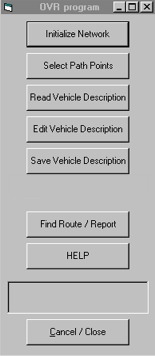
Figure 4. External VB program. Main toolbox.
During a typical run of the routing application, both ArcView and the OVR program, may act as Client or Server depending on the stage of execution.
For example, after pressing the OVR button, ArcView (client) launches the OVR program (server) and establishes a DDE conversation between each other. By pressing some buttons in the OVR toolbox, the OVR program (client) requests ArcView (server) to run scripts to initialize the network or retrieve the location of the path points or find the shortest path.
As mentioned before, a VB application can easily communicate directly with BRINSAP database in Access format. When the OVR program is launched, a communication channel opens the table with corresponding bridge records (BRGON table containing On-system bridges). To rapidly access and retrieve the attributes (number of spans, span length, ratings, etc.) of a specific bridge record, BRINSAPs structure number field is previously indexed. The index is defined outside and before opening the routing application.
The considerable advantage of accessing the bridge attributes in BRINSAPs original format is that any updates to the attributes of the bridges will immediately be accounted for in the routing analysis. The only drawback is that if some bridges are removed from the On-system table (BRGON), because they were closed to traffic or assigned to the Off-System jurisdiction, and the relational database between the roads network and BRINSAP is not updated accordingly, those bridges will not be accounted for in the routing analysis. Therefore, the version of BRINSAP must coincide with the one used to develop or update the network.
To run a typical case, the following items are required:
ﺓ
ArcView
software v3.0a or later,
ﺓ Network Analyst extension v1.0a or later,
ﺓ ArcView project [e.g. Texas.apr] *,
ﺓ Customized extension [OVR.avx] that loads the OVR button, used to launch the external program,
ﺓ External program executable [OVR.exe], and
ﺓ BRINSAP database (in Access format); version should correspond to current roads network.
* The ArcView project consists of a view that contains the required themes for routing analysis (ROADS and OD), and any additional themes that aid in the identification of geographic features (e.g. BRINSAP bridge locations, Political boundaries, Streets, etc.) and the customized scripts (see Figure 5).
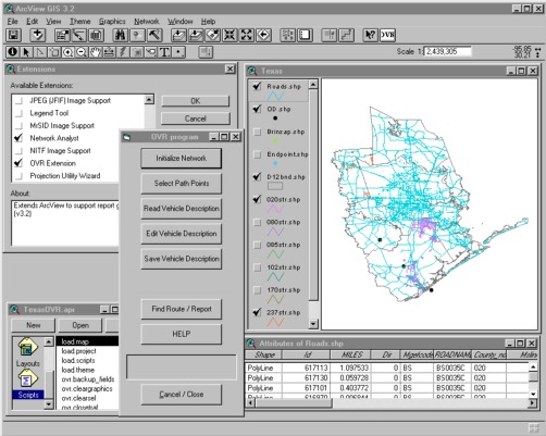
Figure 5. Routing application interface.
The main steps have been listed
in the Steps to Solve a Routing Problem section. The following
paragraphs provide detailed information on each of the tasks performed after
pressing the buttons in the toolbox.
Project initialization
Once the project is opened, clicking on the OVR button begins the initialization of the project. This includes:
ﺓ
Verifying
the presence of the themes needed to generate the network and define the path
points (Roads and OD);
ﺓ
Removing
unwanted path themes (k_shp_xx.shp) created on previous runs that might have
been saved to the OVR project;
ﺓ
Preparing
the Roads theme with the required fields and field names, to facilitate the
extraction of information, and open the corresponding attributes table.
ﺓ
Establishing the cost units.
ﺓ Launching the external program and establishing the DDE communication
A soon as the toolbox is displayed on the screen, two events take place:
ﺓ
A communication
channel with the BRINSAP database is opened, and
ﺓ Vehicle configuration and other variables are initialized.
Initialize the
Highway Network
After project initialization and the OVR program has been invoked, the first step towards solving a routing problem is to initialize the highway network. The network initialization consists in:
ﺓ Generating/regenerating the highway network topology.
ﺓ Enabling road segments that were closed to traffic in previous runs, and
ﺓ Identifying the cost field from which the total cost route will be reported. The default cost is the length of the road segment.
During network initialization, the existing graphics representing trial
routes generated in previous runs (if any) are deleted from the view and table
records currently selected are deselected to initialize the Roads table.
A status message is displayed in the panel after the network has been initialized.
Selection of Pathpoints
The location of the origin and destination of the vehicle needs to be specified to be able to start searching for a route. The OD theme is included for definition of the location of the pathpoints.
To define the location of the pathpoints, the OD
point theme must be selected as the working theme and checked accordingly to
enable viewing of the points that (will) represent the OD pair.
Enable editing capabilities to the OD theme, to
add or modify the location of the path points, using ArcViews tools. Zoom in or out as needed. Save the edits on the theme to account for
them in the routing analysis (see Figure 6).
This version of the program does NOT support "intermediate" stop points where the vehicle could pass through, before reaching the specified destination.
The retrieval of the geographic coordinates of
the path points is accomplished through a customized script in ArcView, which
is executed when clicking on the Select Path Points button in the toolbox.
For every new problem to be solved, the location of the path points must be defined and retrieved.
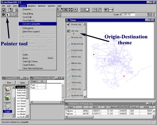
Figure 6. Pathpoint selection.
Vehicle Information
Next, a description of the characteristics of the vehicle is
required. Two options are available:
1.
Read the
vehicle description from an existing file.
2.
Enter a new
vehicle description or modify an existing file.
If the first option is selected, the user is prompted to select an
existing text file with the vehicle information.
By selecting to edit the vehicle description, several dialog boxes may
appear prompting the user for pertinent data.
Initial data includes: vehicle model, type, nominal capacity, height,
width, total number of axles and the selection of an impact factor associated
to the speed at which the vehicle is expected to cross the bridges. See the BLF Evaluation Procedure
section for detailed information on the impact factor. The vehicle's total number of axles includes
the tractor's axles as well as the trailer's. The parameters in these boxes are initialized if a new vehicle
description is to be entered.
The axle configuration information consists of: distance from the
previous axle (zero for the first or steering axle), total axle weight, number
of tires in the axle, axle gage, and tire width (all tires per axle are assumed
to have the same width). The axle gage
is the distance measured between the centers of gravity of the two tire groups.
If a new vehicle description has been entered or an existing description modified, the information can be saved to a text file, by clicking the "Save Vehicle Description" button (see Figure 7).
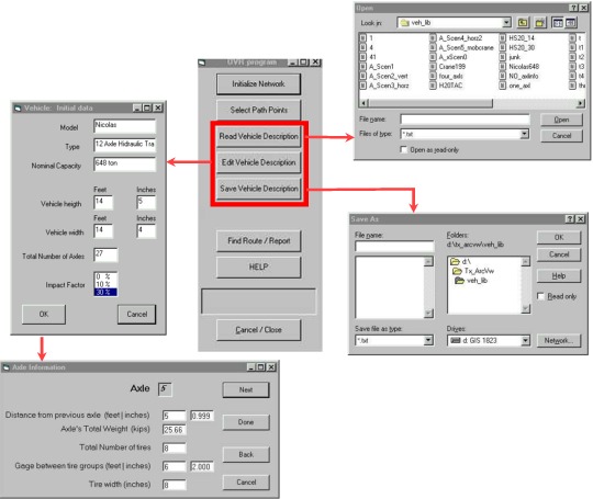
Figure 7. Vehicle
information edit boxes.
Route Search and Report
Once all the above steps have been executed, the
search for a route that meets all clearance and weight conditions may be
initiated.
To start searching for a route, verify that the
Roads theme is the active theme, then press the Find Route / Report button
and select an output file to write the search results. Some activity will be noticed in both
ArcViews interface and the OVR programs panel. In ArcView, each time a shortest path is found, the records
corresponding to the selected road segments are highlighted in the Roads
attributes table, and a graphic representing the selected route is drawn on the
view. In addition, a new path theme is
added to the view.
The OVR program retrieves attribute information
from the Roads table, pertaining to each record that corresponds to the path
under evaluation. This information
includes the structure numbers of the overpass and/or underpass bridges (if
any). Then BRINSAP is accessed to
retrieve the corresponding bridge attributes (e.g. number of spans, span
length, operating rating, etc.) for further evaluation. Several messages appear on the panel,
reporting the status of the bridge evaluation (e.g. evaluation for vertical
clearance, for horizontal clearance, evaluation of TAC requirements or Bridge
Load Formulae, etc).
If a clearance or weight capacity condition is
not met, the corresponding road record is closed to traffic. If a route does not meet the criteria, the
process iterates and a new search is initiated. The network topology is re-generated to account for any road
segments closed to traffic (see Figure8).
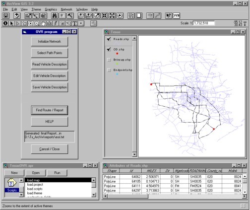
Figure 8. Typical route
search case.
When the routing program finishes the route
searching process, two possible outcomes can be expected:
1. A route is found that
meets the specified constraints.
2. A route is NOT found for
the specified vehicle and path points.
If a feasible route is found, the path is
highlighted (in randomly chosen colors).
In either case, a final report is generated.
At this point, the run is completed and the user may choose to exit the application or continue with another case.
The final report can be viewed
using WordPad or NotePad. Three main sections can be identified in a
typical routing report.
The first section at the beginning of the report describes the vehicle configuration and dimensions, reports the impact factor selected and reports the computed center of gravity of the total vehicle load.
The next section describes the results of the route search, including
the geographic coordinates of the origin and destination pair specified on the
view. The description for a found route
includes headings, highway ID's, mileage, and the cumulative mileage. If a route was not found, the possible
reasons are reported in the following sections. The total number of trial
routes tested before the OVR application gives a result is also reported.
The third and final section includes a list of disabled links with bridges that were avoided due to the different insufficiencies or problems encountered during the search. Depending on the type of problem encountered, the information is classified in five different categories:
a)
Bridges avoided
due to insufficient vertical clearance.
b)
Bridges avoided
due to insufficient horizontal clearance.
c)
Bridges avoided
due to insufficient weight capacity.
d)
Bridges avoided
due to missing information in BRINSAP, and
e)
Bridges avoided
due to Load posting according to BRINSAP.
The application does not
include turn-penalty (intersections where long vehicles might be unable to make
sharp turns) nor restricted access information (road sections under repair or
closed to traffic for other reasons). The disadvantage of not having this
real-time information implemented is that the program may find unrealistic
routes.
This paper documents the development of an ArcView application for routing of super-heavy and oversize vehicles using the Network Analyst extension. The procedure uses a network representation of a system of roads and bridges to identify feasible routes. The route evaluation methodology is consistent with Texas Administrative Code regulations and uses bridge load formulae (BLF) to further analyze load-capacity to expedite the heavy/oversize vehicle permit process. The application utilizes vehicle and bridge information to automatically search for the shortest path between an origin and a destination, closing to traffic all road segments with inadequate bridges and locations of restricted clearances.
The routing application features an external program, developed in Visual Basic that interfaces between ArcView and the bridge database.
Problems with geographic information sources, interface details and a typical run are addressed. Inclusion of restricted access and turn-penalty information is yet to be implemented.
This project was funded by the Texas Department of Transportation under studies 0-1482 and 0-1823. The authors wish to express their appreciation to Mr. John Holt, Mr. Mike Lynch and Mr. Will Watson from DOT for their invaluable and continuous support.
A very special thanks to the NAFTA Intermodal Transportation Institute for providing additional financial assistance to continue this research, and to the Center for Highway Materials Research for supporting and encouraging this work.
The authors would also like to acknowledge Dr. Alberto Garcia-Diaz from Texas A&M University, Dr. Cesar Carrasco and Dr. Suleiman Ashur from UTEP for their valuable contributions during the early stages of the research.
Finally, to all the graduate and undergraduate students who participated, for their patience in the laborious tasks.
[1] Texas Administrative Code, 1992 Supplement, West Publishing Co., St. Paul, MN, (1992).
[2] P.B. Keating, "Overweight Permit Rules," Research Report 1433-IF, Texas Transportation Institute, Texas A&M University, College Station, TX. (1994).
[3] R.A. Osegueda, et al., "Development of Automated Routing of Overweight/Oversize Vehicle System for Houston District," Report TX-96-1482-1, The University of Texas at El Paso, TX, April 1997.
[4] R.A. Osegueda, et al., "GIS-Based Network Routing Procedures for Overweight and Oversize Vehicles," Journal of Transportation Engineering, July/August 1999.