Design and Implementation of a Data-Centered Groundwater Modeling System
Bruce Rindahl, P.E. , Principal Engineer, Brown and Caldwell
Ray Bennett, P.E. , Manager of Special Projects, State Engineers Office, State of Colorado
Abstract
As part of a decision support system for the Rio Grande basin, the State of Colorado has designed and implemented a data-centered interface for groundwater modeling. The new interface includes spatial GIS data, the State's relational database, the USGS MODFLOW groundwater model, and several planning and analysis models for water administration. In addition, the interface has provisions for display of groundwater results using a variety of tools including ArcView GIS and ArcExplorer.
This paper will describe in detail the development and implementation of the data-centered interface to groundwater modeling, with particular emphasis on the GIS interaction between the various data sources, models, and display and analysis of results.
By using the existing models and a data-centered approach, the interface has been designed as a versatile system, responding to revised and updated data, comparing historic conditions to potential future scenarios, and allowing interaction and iterations between surface and groundwater models.
Introduction
The Rio Grande Decision Support System (RGDSS) is currently under development by the State of Colorado as part of a series of decision support systems for the analysis and administration of water. These decision support systems are collectively called the Colorado Decision Support System (CDSS). Several components were previously developed by the state including HydroBase, a relational database containing water rights, diversions, and all other records of water administration. One of the major goals of the CDSS is to create programs, models, and interfaces that are data centered, that is they must be dependent only on the data stored in HydroBase and other sources. They also must be transferable to other basins in the state with a minimum of effort.
The major new component created in the RGDSS is a groundwater modeling system to analyze the movement and impact of well pumping on the surface water system in the Rio Grande basin. This groundwater modeling system must also be data centered in it depends on information in HydroBase, output from other models of the CDSS, and basin specific data developed in a systematic manner.
Approach
The procedures used to design and develop the data centered ground water modeling system for the Rio Grande basin was as follows:
Historic Simulation Procedure
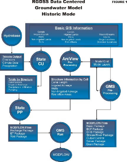
The procedures for preparing an historic data set using a data centered groundwater modeling process is presented in Figure 1 and consist of the following 5 steps.
Step 1. Develop Basic GIS Coverages
Step 2. GMS Modeling Interface
Step 3. ArcView Data Analysis
Step 4. StateCU Analysis
Step 5. State Preprocessor
Step 1. Develop Basic GIS Coverages
For the basin in question, general GIS coverages will be developed from various sources of information. The coverages developed for the RGDSS for the data centered groundwater model include Rivers/Streams, Canals, Drains, Surface Irrigated Lands, Groundwater Irrigated Lands, Wells, Non-Irrigated Lands, Soils, Rim Inflows, Diversion Locations, and Gage Locations. All GIS coverages must be developed on a common datum and consistent units. For the RGDSS the units are meters and the datum is UTM Zone13.
Step 2. GMS Preprocessing Interface
The selected groundwater modeling interface tool, GMS, will utilize the basic GIS coverages to develop the standard input packages to a MODFLOW groundwater model. The outputs from GMS will include the input files required by the following MODFLOW packages:
In addition to the standard MODFLOW packages, GMS will export the model cell grid system as a DXF export file. This file will be translated into a shapefile by a script developed in the ArcView Data Analysis (Step 3) for computing individual properties of such parameters as irrigated lands, canal leakage, and precipitation on a cell-by-cell basis. Detailed examples of the output files and formats can be found in the documentation for the GMS software package.
Step 3. ArcView Data Analysis
The GIS coverages from Step 1 and the model grid DXF file developed by the GMS modeling interface in Step 2 will be used by an ArcView GIS application. This application will develop five (5) output files for use by the SPP to compute information on a cell-by-cell basis. This application, called StateDGI, written in ArcView's Avenue scripting language and Microsoft Access, will detail for each structure the cells that are associated with a particular groundwater flux term (deep percolation, pumping, canal recharge, evapotranspiration, and pumping). For example, a ditch system or structure may provide ground water recharge via canal leakage to one or more ground water cells. Similarly, a structure may provide ground water recharge via deep percolation from irrigated lands to one or more model cells. Other ground water flux terms that have a spatial component include well pumping, precipitation recharge on non-irrigated lands and rim inflows. In addition, StateDGI will allow groundwater flux terms to accrue to layers other than the upper layer. For example, some of the rim inflow areas may recharge separate layers in the groundwater model.
These output files will be used by the SPP in Step 5 to develop input data for the MODFLOW program. Note that, in general, the ArcView data analysis is required only once for a particular basin and model grid configuration. This is because the output files are independent of the flux quantity, the time period being modeled and the number of time steps being simulated. However, if the basic spatial data does change (e.g. the model grid is revised, irrigated acreage cannot be assumed constant, additional canals are modeled, etc.) the above process can be repeated easily.
Step 4. StateCU Analysis
The State's Consumptive Use Model, StateCU, performs a water supply analysis of consumptive use (CU) by structure. As part of the CU analysis, StateCU provides canal loss, surface water applied and pumping by structure. It will be enhanced to compute deep percolation from precipitation on non-irrigated lands with native vegetation.
In addition to the parametric CU data (crop coefficients, root zone depth, etc.) the CU model uses historic climate (temperature, precipitation and frost data) and diversion records obtained from State�s central database, HydroBase. It also uses the irrigated lands, soil types, and water supply (surface water only, ground water only or both) from the spatial data developed in Step 1.
The StateCU model will develop time series data for each time step in the study period. As presented in Figure 1, the four (4) output files resulting from the State CU model are as follows:
These output files will be used in Step 5 by the SPP to develop input data for the MODFLOW groundwater model.
Step 5. State Preprocessor (SPP)
The SPP will take the input files developed from the Arc View Analysis (Step 3) and the StateCU Analysis (Step 4) to generate three (3) input files for MODFLOW as follows:
Recharge Package
The Recharge package will be computed by totaling the canal leakage, the deep percolation, rim inflows, and precipitation on non-irrigated lands for the entire basin. Each cell in the groundwater model will accumulate canal leakage and deep percolation for each structure and the accumulated total will output in the recharge package format required by MODFLOW.
Recharge from Canal Leakage
The formula to compute canal leakage for each cell containing a canal or lateral is as follows:
Leakageijk =
Where: i = Model cell row
j = Model cell column
k = Structure number
The values for Lengthijk and Weightijk are obtained from the ArcView data analysis output in the Canal Length file. Values for the TotLeakagek is the total canal leakage for each structure for each time step. The denominator is the sumproduct of the individual length and weight terms from each cell by structure and is output from StateDGI. The SPP will aggregate the monthly leakage data from the StateCU model into any desired time step, such as annual data or a specific time period. Where the canal losses can occur into different layers of the groundwater model, StateDGI will also track lengths for the individual layers.
Recharge from Surface Water Irrigation
The formula to compute recharge from deep percolation for each cell associated with irrigated lands is as follows:
Percolationijk = ![]()
Where: i = Model cell row
j = Model cell column
k = Structure number
The values for Areaijk and Weightijk are obtained from the ArcView data analysis output in the Irrigated Acreage file. Values for the TotPercolationk is the total deep percolation rate for each structure for each time step. The percentage of surface irrigation by structure resulting in deep percolation will be computed by StatePP. The weight field in the irrigated lands coverage could be used for this value to aid in calibration of a groundwater model. The SPP will aggregate the monthly irrigation data from the StateCU model into any desired time step, such as annual data or a specific time period. Note that the deep percolation associated with irrigated lands includes percolation from precipitation falling on irrigated lands during the non-irrigated season. Where the deep percolation can occur into different layers of the groundwater model, StateDGI will also track areas for the individual layers.
For the case of irrigated lands being serviced by several ditch systems, a unique irrigated parcel identifier will be included as one of the attributes of the shapefile. StateDGI will compute the areas in each model cell by parcel listing the parcel id and areas in each cell. A table will be developed in Access that lists every structure serving the various parcels and the respective percentage of service. For example, an irrigated parcel served equally by two ditch systems will have two records in the Access table with the structure id�s and percentages of 50% for each. Each record of the table will have a different ID number corresponding to the ditch systems serving the parcel. This table will be similar to or linked to the table irrig_structure in HydroBase. Any number of ditch systems, with any distribution of water supply to that particular field, will be handled in this manner.
Recharge from Rim Inflows
The formula to compute recharge for each cell receiving rim inflows is as follows:
RimInflowij = 
Where: i = Model cell row
j = Model cell column
k = Structure number
The values for Areaijk and Weightijk are obtained from the ArcView data analysis output in the Rim Inflow Areas file. Values for the TotRimFlowk is the total rim inflow for each rim inflow area for each time step. The denominator is the sumproduct of the individual length and weight terms from each cell and is output from StateDGI. The SPP will aggregate the monthly time step data from the StateCU model into any desired time step, such as annual data or a specific time period. Where the rim inflows occur in different layers of the groundwater model, StateDGI will also track areas for the individual layers.
Recharge from Precipitation on Non Irrigated Lands
The formula to compute recharge from precipitation for each cell with native vegetation, non-irrigated lands is as follows:
Rechargeij = ![]()
Where: i = Model cell row
j = Model cell column
k = Native Vegetation Type
The values for Areaijk and Weightijk are obtained from the StateDGI output in the Non-Irrigated Vegetation file. TotPercolationk is the percolation rate for each type of vegetation for each time step. The SPP will aggregate the monthly percolation data from the StateCU model into any desired time step, such as annual data or a specific time period. Where the infiltration from native vegetation occur in different layers of the groundwater model, StateDGI will also track areas for the individual layers.
Total Recharge
The total recharge for each cell is the sum of the canal leakage, deep percolation, rim inflows and native percolation computed from the above steps and a output file in the standard MODFLOW format for the recharge package is created by the SPP. Note any cell in the groundwater model can have components from any or all of the above sources. For example, a cell can include irrigated lands covering 75% of the area of the cell, along with 10% covered by native vegetation and 15% rim inflows. Since the output from the StateCU will be infiltration rates, the total recharge will be the sum of the various rates multiplied by the associated areas.
ET Package
The ET package for the data centered ground water interface will be developed by the StatePP for use in a MODFLOW groundwater simulation. This package will be developed from the cell by cell ET zones output from StateDGI, evapotranspiration characteristics for each type of native vegetation, and estimated precipitation recharge on native non-irrigated vegetation for the basin. The StatePP will estimate ET rates for each type of vegetation along with the estimated extinction depths at each cell.
It should be noted the ET package may not be included in preliminary runs of a groundwater simulation. Once several iterations of a particular model have been run and appear to be stable, the ET package will be included for calibration purposes both to compare to measured heads and to the estimated ET from the water budget component of the StateCU model.
Well Package
In order to associate the irrigated lands with one or more wells serving them, a spatial comparison between the irrigated lands and the final well coverage was performed. A parcel is estimated to be served by groundwater if the parcel was irrigated by sprinklers or has an irrigation well located within the parcel. The procedure to match irrigation wells with groundwater irrigated parcels is as follows:
It is anticipated that all parcels served by groundwater will have a physical well assigned by steps 1 - 3 or an estimated well assigned by step 4. Figure � 1 shows an example of the various parcel and well combinations described in steps 1 � 4 above. The results of this well to parcel matching program will be a table in Access that gives the unique well id, the associated parcel id, the type of match made (1 � 4) and the distance from the well to the parcel where applicable.
Methods and Types of Well Assignments
In addition to assigning irrigation wells to groundwater irrigated parcels, StateDGI will estimate the distribution of pumping for each well by model layer. The layers defining the bottom elevation are input to the StateDGI. The first layer is a ground elevation grid in ArcView format for the model area, and each subsequent layer is a bottom elevation grid for that respective layer in ArcView format. Attributes for each well obtained from HydroBase are used to define the percentage of well capacity from each well layer. The procedure to determine the pumping distribution for each well is as follows:
The results of this well layer program will be a table in Access that gives the unique well id, the layer number, the percentage of pumping from that layer, and the well id of the closest well found in step 4 above if applicable.
The final result from all of the well analysis is a text output file from Access. Groundwater pumping by structure and time step will be estimated by StateCU. To compute pumping to each individual well, the following procedure is used. Divide total pumping from StateCU by Total_Weighted_Acreage for that structure. This will give an application rate in AF/Acre (assuming StateCU gives pumping volumes in AF). For each parcel multiply the pumping rate by the Weighted_Area for that parcel to give a pumping volume for the parcel. To compute the final pumping volume for each well, prorate the pumping volume for the parcel by the capacities of each well serving that parcel. These pumping volumes for each well will then be input to the groundwater model by StatePP by model layer, row, and column.
The year field for each well will be used to selectively shutdown wells during a time step prior to their construction. StatePP will need to compute the total capacity of the active wells to distribute the pumping as well as the reduced groundwater acreage if a parcel has no active wells.
The sum of the parcel acreage may not add up to the value in the Total_Acreage and the Weighted_Acreage fields. This is because some of the irrigated lands and wells are not in the model grid. StatePP will have to use the values in the Total_Acreage and the Weighted_Acreage fields for the accurate pumping rates.
Future or What-If Simulation Procedure
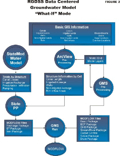
The procedures for preparing a future or What-If data set using a data centered groundwater modeling process is presented in Figure 2 and consist of the following 5 steps.
Step 1.* Develop Basic GIS Coverages
Step 2.* GMS Modeling Interface
Step 3.* ArcView Data Analysis
Step 4. StateMod Analysis
Step 5.* State Preprocessor
*Identical to Historic Data Preparation
The steps outlined in the historic data procedure will create a data centered groundwater model for a historic period of simulation. In order to simulate potential future situations, or a "What-If" scenario, the StateMod surface model will used in Step 4 instead of the StateCU model. The State CU Water Model is designed to simulate a river basin using the prior appropriation doctrine. Results include estimated streamflows, diversions, and reservoir operations under a user provided set of operating rules. Note that the StateMod will be enhanced to include a groundwater component as part of RGDSS. The StateMod model will develop similar time series data for each time step in the study period. As presented in Figure 2, the four (4) output files resulting from the StateMod are as follows:
These output files will be used in Step 5 by the SPP to develop input data for the MODFLOW groundwater model. Identical information will be created for input to the StatePP for development of a groundwater model reflecting the future or "What-If" scenario created using the StateMOD model.
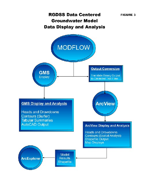
Model Runs and Display Results
The GMS software package has an interface to select the various model packages required by MODFLOW, run the selected model, and save the various output files from the model. The data centered ground water modeling process includes two methods of viewing and analyzing results; the GMS Output Interface and the GIS Output Interface. The GMS software package used in the preparation of the groundwater model also has several features for display and analysis of the results of a model run. Unfortunately, GMS software package is a proprietary program whose cost could be prohibitive to other users. Because of this a secondary form of displaying MODFLOW results will be developed. This secondary approach will use ArcView to display results of the MODFLOW program directly in the ArcView interface and thus can develop shapefiles for use by ArcExplorer.
GMS Output Interface
In addition to the data preparation functions of GMS described previously, the GMS modeling system will be used to preview input data, summarize results, plot contours of various model results such as final heads and drawdowns, and print results in a tabular display. Some of the functionality included in GMS are contour maps of various drawdowns and heads for each time step, summary tables and report output from the MODFLOW files. Complete details of the GMS software package are included in the documentation of that program. Unfortunately, GMS is a propitiatory piece of software that may not be readily accessible to many RGDSS users.
GIS Output Interface
Results of all MODFLOW model simulations will also be converted into tabular form for use by users of ArcView and ArcExplorer. This will allow the display and analysis of the groundwater simulations by users without requiring the purchase of the proprietary software package GMS. As opposed to GMS, the ArcView data viewing allows model results to be joined to the model grid. The procedure will join the tabular form of the MODFLOW output to the model grid shapefile developed in Step 2 of the modeling procedure. Thus the results of the simulation will become a part of the attribute table for the individual cells.
This allows the complete analysis and display of the results of various runs performed as part of the RGDSS. With appropriate tools in ArcView, GIS users can also create such secondary information has contour mapping, differential analysis between various runs, maximum drawdowns, etc. This allows full functionality of the GIS software package to analyze results of the groundwater modeling effort.
In addition to viewing the results using ArcView, the model results joined to the model grid can be exported as a complete shapefile. This will allow the complete analysis of the various runs to be contained in the attribute table of the shapefile. The shapefile can be placed on the CDSS Web site and can be downloaded for use by ArcExplorer. While ArcExplorer does not have the full functionality of ArcView, it can display numerous features of the results including heads and drawdowns for each time step of the model. ArcExplorer is a GIS software package that is freely available from the manufacturer. In this manner, the groundwater model results can be viewed by anyone without requiring the purchase of any software package.
Summary
A data centered approach has been designed for the groundwater modeling component of the RGDSS. This approach will utilize both existing models and new routines developed specifically for the RGDSS. Based on the original preprocessor developed by the State of Colorado in 1991, the new interface includes GIS data, the selected groundwater modeling interface, GMS, the existing tools from HydroBase, the results of StateMod simulations, and the CU/Water Budget from the RGDSS.
By using the existing models and a data centered approach, the interface is designed as a versatile system, responding to revised and updated data, refinement of specific models, comparing historic conditions to potential future scenarios, and allowing interaction and iterations between surface and groundwater models.
Authors
Bruce Rindahl, P.E.
Principal Engineer
Brown and Caldwell
7535 E. Hampden Ave.
Denver, Colorado 80231
Ray Bennett, P.E.
Special Projects Manager
Division of Water Resources
1313 Sherman Street, Room 818
Denver, Colorado 80203
ray.bennett@state.co.us