Figure 1: LINETRACE 30-meter
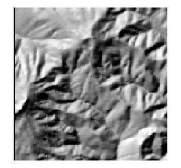
Figure 2: 30-meter resampled to 10-meter
TopoTools consists of 5 AMLs that augment the capabilities of ArcINFO in the area topographic modeling. The tools are named ENFORCE, STREAMLINE2, SLOPEPOSITION, VISIBILITY2, and ZONALGEOMORPH. Some contain C, JAVA, and/or FORTRAN programs.
How many of you like Esri GIS tools? I have a confession, I don't.
The reason is
that most of them work! (for the most part) and they provide a wide variety of GIS
functionality. As a GIS programmer I no longer have as many fun projects. ;-( However,
there are still some things that Esri products don't do, or don't do the way we want
them to. This is why the TopoTools were written.
enforces the valley and ridgelines in an elevation grid generated from contours. Background: Some processes that create DEMs from contour data create unnatural terracing, especially along valleys and ridgelines (i.e. places with greater curvature). The ENFORCE tool minimizes this terracing by smoothing the DEM along flow lines (both downhill flow lines, i.e. valleys, and uphill flow lines, i.e. ridges), while still adhering to the source contours.
_______________________________________________________________________ENFORCE <in_grid> <out_grid> <contour_interval> {z_factor} {iterations} {FLAT | NOFLAT} {locking_factor} {flow_min} {NOCURVE | CURVE}
Digital Elevation Models (DEMs) exist for all or most of the United States at 30-meter resolution. However, the 30-meter DEMs don't contain a lot of detail when viewed at a small scale.
Figure 1: LINETRACE 30-meter |
Figure 2: 30-meter resampled to 10-meter |
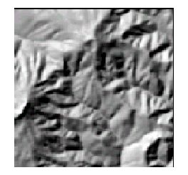
Figure 1 is a hillshade of a 30-meter DEM created using LINETRACE software. This DEM came from the US Geological Survey (USGS). LINETRACE creates DEMs by interpolating elevations between contour lines. The area displayed is roughly 2x2 miles in size. Figure 2 is a hillshade of the same DEM after it was resampled to 10-meter cell size. The image is a little sharper.
In order to retain more detail the USGS and US Forest Service (USFS) are now having 10-meter DEMs created from the contour lines (i.e. not just by resampling the 30-meter data.)
Figure 3: LINETRACE 30-meter |
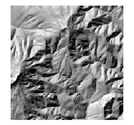 Figure 4: LT4X 10-meter |
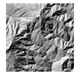 Figure 5: TOPOGRID 10-meter |
Figure 3 is the 30-meter created using LINETRACE software. Figure 4 is a 10-meter DEM created using LT4X software (Averstar, Inc.) This came from the USFS. L4TX, like LINETRACE, creates DEMs by interpolating elevations between contour lines. There's a lot more detail in the 10-meter DEM than in the 30-meter DEM or the resampled 10-meter DEM (Figure 2). However, not all of this extra detail looks good. The most notable example is the terracing which is most noticeable along some if the valley bottoms and ridgelines. Figure 5 is a hillshade of a 10-meter DEM created from contours using the TOPOGRID command in ARC. It also exhibits the terracing.
So is this terracing real? Some of it probably is, but most of it probably isn't. So where it's not real, is this a result of a limitation in the source contours or in the DEM creation software? It's a limitation of both.
There are different types of terracing. One way to categorize terracing is in two categories: terracing between contour bands (i.e. inter-band terracing), and terracing within contour bands (i.e. intra-band terracing.)
INTER-BAND terracing is a result of irregularly spaced contours. Some of this certainly reflects reality, but some probably doesn't and is instead a result of how the contours were drawn. DEM generation algorithms can reduce some of this by letting the contours "float" a little, but in so doing some good detail may be lost. In general I consider inter-band terracing (that doesn't reflect reality) to be a limitation of the source contours.
INTRA-BAND terracing is where terracing exists within a contour band. In other words, both the flat and the steep part of a terrace exist between two contour lines, and this pattern repeats itself from one contour band to the next. This terracing is not indicated in the contours, and is thus a limitation of the DEM generation algorithms.
So why do the algorithms create intra-band terracing? One reason is because they are biased in favor of the "concave contour".
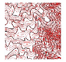 Figure 6: LT4X 10-meter |
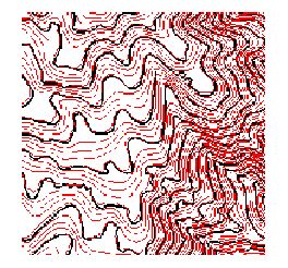 Figure 7: TOPOGRID 10-meter |
Figures 6 and 7 show 10-foot contours (in red) that were generated from the 10-meter DEMs. The DEMs themselves were generated from 40-foot contours (in black). Generating and displaying intermediate contours like this is a good way to see the terracing, and it shows the "concave contour" biasing. Both along valleys and ridge lines, on the inside (or concave side) of curves in the 40-foot contours, the 10-foot contours are more widely spaced. Therefore, the 10-meter DEMs are flatter is these areas, and they are closer in elevation to the concave contour then to the adjacent convex contour. Conversely, on the outside (or convex side) of the curves, the 10-meter DEMs are steeper. There is nothing in the source 40-foot contours to suggest that such a terracing pattern exists. In this way, the algorithms are biased in favor of the "concave contour".
It's understandable how concave-contour biasing occurs. In the case of LT4X it runs profile lines through each point in the DEM, intersecting these lines with the neighboring contour lines, and using this information to interpolate an elevation for the DEM point. The profile lines are more likely to intersect the concave contour that wraps around the DEM point, then they are to intersect the convex contour bending away from the point. Moreover, the intersection is more likely to be closer to the concave contour. In this way, concave-contour biasing is not surprising.
ENFORCE was written to reduce the terracing, while still adhering to the source contours. It is an AML driven program. The premise from which it was designed is that terracing isn't much of a problem when break lines along valley and ridgelines are included with the contours when the DEMs are created. In fact, most of the 10-meter DEMs being produced by the USGS and USFS are "drainage enforced", i.e. streams are used as break lines. However, the USGS and USFS have been only using mapped streams, and there are a lot of valley crenulations without mapped streams. Moreover, break lines along ridges have not been used.
What ENFORCE does is generate break lines from the DEM using the streamline generation tools in GRID module of ArcINFO. Streamlines are generated the normal way, and then the DEM is inverted and ridgelines are generated. Next these break lines and the source contours implied by the DEM are used to create a new DEM by fitting a smooth surface to this wire frame. A program outside of ArcINFO performs this step.
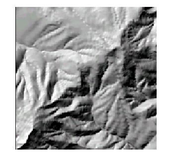 Figure 8: LT4X 10-meter |
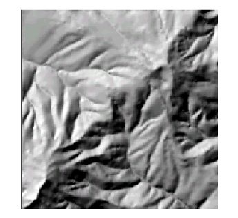 Figure 9: After ENFORCE |
Figures 8 and 9 show how ENFORCE is successful at reducing the terracing. The improvement is even more noticeable in a map of slope (Figures 10 and 11.)
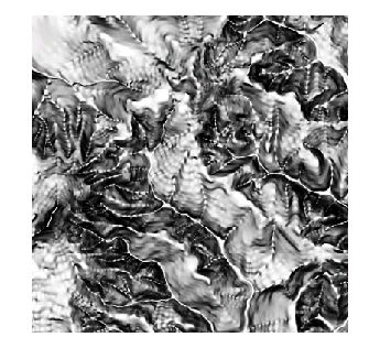 Figure 10: LT4X 10-meter |
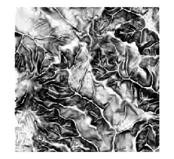 Figure 11: After ENFORCE |
Yet another way to look at the difference is by displaying the intermediate contours generated from the DEMs.
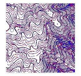 Figure 12: Before (red) vs. After (blue) |
Figure 12 shows how ENFORCE creates a more constant gradient along valleys and ridgelines, which is more realistic. It also shows how ENFORCE adheres closely to the source contours. There are some discrepancies, but using the default {locking_factor} of 1 can reduce these.
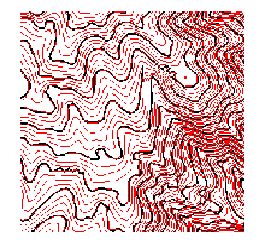 Figure 13: Locking factor = 0 |
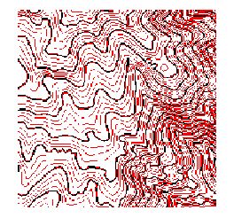 Figure 14: Locking factor = 1 |
Using a {locking_factor} of 1 (Figure 14) results in a better fit with the source contours, but results in slightly less reduction of terracing, as can be seen in slope maps (Figure 15 and 16.)
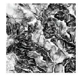 Figure 15: Locking factor = 0 |
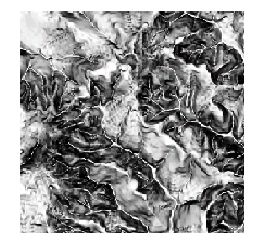 Figure 16: Locking factor = 1 |
ENFORCE can be used to improve 10-meter DEMs being generated by the USGS and USFS. In general it increases the DEMs appearance and accuracy, in respect to elevation and slope.
Limitations: However, in respect to planar curvature (e.g. as measured along a contour line), ENFORCE decreases the DEMs accuracy by slightly increasing curvature (see Figures 12 and 13.) Another limitation with ENFORCE is that the DEMs it produces occasionally don't follow the drainage enforcement in the input DEM. This can happen in flat areas, e.g. flood plains.
creates a stream coverage from a surface grid using GRID functions in conjunction with outside programs to determine flow direction. The outside programs are better than GRID FLOWDIRECTION for the purpose of creating stream networks.
________________________________________________________________________STREAMLINE2 <in_grid> <out_cover> {fdir_grid} {stream_grid} {cellsize} {fill_limit} {flow_min} {NOORDER | STRAHLER | SHREVE} {weed} {REGULAR | RANDOM} {FLAT | NOFLAT}
Streamlines are located by tracing the direction of flow over a surface grid. STREAMLINE2 does this in a similar manner as is described in "Surface hydraulic analysis" under "Cell-based Modeling with GRID" in ArcDoc. However, STREAMLINE2 employs two outside programs, RESAMPLE2 and FLOWDIRECTION2, which lead to better results in areas where stream crenulations are not well defined.
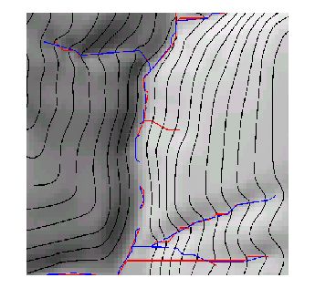 Figure 17: ArcDoc technique (red) vs. STREAMLINE2 (blue) |
RESAMPLE2 - First the <in_grid> is resampled to {cellsize}, as long as {cellsize} is smaller than the cell size of <in_grid>. Resampling is done using RESAMPLE2, a FORTRAN program. RESAMPLE2 calculates new cell values by interpolating on a triangular regular network (TRN) (see Geographic Information Systems and Cartographic Modeling, C. Dana Tomlin, 1990, fig 1-21). This method may be no more accurate than the methods used by GRID RESAMPLE, but it works better in conjunction with FLOWDIRECTION2.
FLOWDIRECTION2 - After sinks are filled, then flow direction is calculated. This is done using GRID FLOWDIRECTION and FLOWDIRECTION2, a FORTRAN program. FLOWDIRECTION2 combines the results from GRID FLOWDIRECTION with flow direction values calculated in a different manner. Flow direction is the direction of greatest descent away from a cell.
GRID FLOWDIRECTION considers just the 8 cardinal directions, to the 8 neighboring cells, when determining flow direction. Flow direction in reality is not limited to the 8 cardinal directions, thus the results from GRID FLOWDIRECTION are limited.
On the other hand, FLOWDIRECTION2 calculates flow direction from each cell over the 8 triangles formed between the cell and it's 8 neighbors. This preliminary calculation can yield any direction, not just the 8 cardinal directions. Then the results are reduced to the 8 cardinal directions by means of percentages. For instance, when the preliminary calculation is 25 degrees, then roughly 50% of the time this cell will be assigned a value of 64 (0 degrees, North) and roughly 50% of the time it will be assigned 128 (45 degrees, Northeast). When averaged over many cells, this will approximate a flow direction of 25 degrees. This is why resampling to a smaller {cellsize} improves the results.
In this way, FLOWDIRECTION2 in conjunction with RESAMPLE2 lead to a more accurate determination of flow direction, which in turn yields more accurate streamline generation, especially where stream crenulations are not well defined. For example, see the two streams flowing East to West in the bottom of Figure 17.
However, FLOWDIRECTION2 does supplement its results with the results from GRID FLOWDIRECTION. It also relies on the results from GRID FLOWDIRECTION where the determination of flow direction used by FLOWDIRECTION2 would result in crisscrossing streams.
{FLAT | NOFLAT} - Another enhancement in STREAMLINE2 is the treatment of flat areas. By default, approximate center lines are drawn through flat areas. This is slower than relying on GRID FLOWDIRECTION, but it is more realistic. In flat areas, GRID FLOWDIRECTION can yield a solid mass of streams that looks more like a computer chip.
In most areas, streamlines generated using the process defined in ArcDoc are very similar to streamlines generated by STREAMLINE2. However, where stream crenulations are not well defined (e.g. headwaters or flat valleys), STREAMLINE2 is more accurate.
creates a grid of slope position from a grid of elevation. Values in the output grid range from 0 (valley floor) to 100 (ridge top).
________________________________________________________________________SLOPEPOSITION <in_grid> <out_grid> {sink_fill_limit} {peak_fill_limit} {valley_accum_min} {ridge_accum_min}
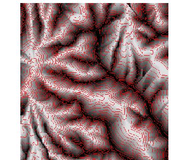 Figure 18: Slope Position Generated from DEMs |
CALCULATING SLOPE POSITION - Slope position of cell is its relative position between the valley floor and the ridge top. Results depend on the limits used for the arguments. Therefore, it is recommended to test SLOPEPOSITION on a small area first.
FILL SINKS AND LEVEL PEAKS - Sinks and peaks that are smaller than user specified limits are filled and leveled, respectively. This is done by means of the FILL command in GRID.
The reason for removing small sinks and peaks is to make the valleys and ridges fairly continuous. Otherwise, each little sink and peak will become a dead end, breaking the valleys and ridgelines when they are identified via FLOWACCUMULATION.
However, removing sinks and peaks does remove definition from the data, so care should be taken not to use too large a z_limit ({sink_fill_level} and {peak_fill_level}). For example, removing peaks is equivalent to chopping of the peak at the elevation of its highest saddle. Once this is done the whole leveled area is treated the same, and any definition between its flanks and top are lost.
IDENTIFY VALLEYS AND RIDGELINES - Downhill and uphill flow accumulation values greater than user specified limits are used to identify valleys and ridges, respectively. Flow accumulation is calculated using the FLOWDIRECTION and FLOWACCUMULATION commands in GRID.
The specified limits ({valley_accum_min} and {ridge_accum_min}) determine the scale at which slope position will be calculated. For example, when large limits are used only large valleys and ridges will be identified as such, and small valleys and ridges will be considered somewhere mid-slope.
CALCULATE SLOPE POSITION - Slope position is calculated for the cells in the output grid as the elevation of each cell relative to the elevation of the valley the cell flows down to and the ridge it flows up to. This is represented as a ratio, ranging from 0 (valley floor) to 100 (ridge top). The formula is:
slopeposition = INT ((cell_elev - valley_elev) / (ridge_elev - valley_elev) * 100 + .5)
performs visibility analysis on a grid. VISIBILITY2 is similar to GRID VISIBILITY with some notable exceptions. VISIBILITY2 is generally much faster (about 10 times) and, in addition to FREQUENCY, has a MAGNITUDE analysis option. MAGNITUDE not only takes into account the number of observation points visible from a cell, but also the size that the cell appears to be from the observation points. However, VISIBILITY2 does not support all the options that GRID VISIBILITY does.
________________________________________________________________________VISIBILITY2 <in_grid> <out_grid> <cover> {POINT | LINE} {FREQUENCY | MAGNITUDE}
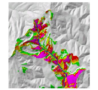 Figure 19: Frequency |
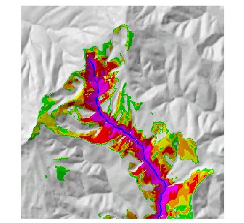 Figure 20: Magnitude |
VISIBILITY2 identifies the area seen from the points in a point coverage, or the vertices of the lines in a line coverage.
The MAGNITUDE option was written for a landscape architect who wanted to be able to take into account not only the number of times that a location is seen (FREQUENCY), but also the distance of the location from the observation point, as well as the angle of the ground at the location relative to the position of the observation point. MAGNITUDE takes into account these 3 factors (frequency, distance, and angle) into one calculation. The output grid records the approximate percentage that each grid-cell location contributes to the total view from the observation points.
To compensate for the cells whose percent contribution to the total view is very small, the MAGNITUDE VALUEs are recorded in 1/1000's of a percent. Thus, if the VALUE of a cell in the output grid is 1000, then this cell takes up 1 percent of the view from the observation points. It follows then that the sum of the VALUEs in the output grid should not exceed 100,000, or 100 percent of the view. In actuality, if you are viewing over topographic data, the sum of the VALUEs will usually be closer to 50,000, or 50 percent of the view, where the rest of the view is occupied by sky and is not counted. When there is more than one observation point, then the VALUE in each cell of the output grid is based on the average percent that the cell contributes to the view from each of the observation points.
To illustrate how MAGNITUDE works, imagine that you are standing at an observation point and that you have a clear globe around your head. OK? Now trace the outline of each visible grid cell onto the inside of the globe. The MAGNITUDE of the grid cell is the percentage that it occupies of the total surface area of the globe.
RESULTS - Figures 19 and 20 show the results of using the FREQUENCY and MAGNITUDE options, respectively, to perform a visibility analysis from observation points along a stream. The differences between the outputs are predictable. Prominent ridges overlooking the stream receive relatively higher FREQUENCY values. They are seen from a lot of points along the stream, but aren't very close to the stream. On the other hand, the lower slopes just above the stream receive relatively higher MAGNITUDE values. They are very close to the stream, but only visible from a few points.
summarizes for each zone of the input zone grid geomorphic calculations of the input elevation grid and records them in the output INFO table. The geomorphic calculations include various measurements of elevation, slope, aspect, and curvature.
________________________________________________________________________ZONALGEOMORPH <zone_grid> <elevation_grid> <output_info_file> {z_factor} {geomorphic_name}
ZONALGEOMORPH packages existing GRID functions.
{geomorphic_name} is the keyword that defines which geomorphic calculations will be performed and summarized by zone. The default is for ALL calculations to be made. Valid keywords are:
| ALL ELEVATION_MEAN ELEVATION_MIN ELEVATION_MAX SLOPE_MEAN SLOPE_MEAN_NET SLOPE_MIN SLOPE_MAX ASPECT_MEAN_NET ASPECT_STRENGTH CURVATURE_MEAN CURVATURE_MEAN_A CURVATURE_MIN CURVATURE_MAX |
All of the following calculations are performed Average elevation Minimum elevation Maximum elevation Average slope Net average slope, taking into account variation in aspect Minimum slope Maximum slope Net average aspect Degree to which aspect is scattered Average curvature Average of absolute value of curvature Minimum curvature Maximum curvature |
Part of the reason for writing ZONALGEOMORPH, as opposed to using existing zonal functions, like ZONALMEAN, is the more complicated nature of aspect and slope. For example, to average aspects of 10 degrees and 350 degrees, using a normal average, the result is ( 10 + 350 ) / 2 = 180 degrees, or due South. But the average should be 0 degrees, due North, so a normal average won't work. Instead, ZONALGEOMORPH uses a vector average. To illustrate, take a vector (i.e. an arrow) that is one unit long and point it at 10 degrees. Next take a second vector of the same length, point it at 350 degrees, and attach its tail to the head of the first vector. Now draw a vector from the tail of the first vector to the head of the second vector. The aspect of this third vector is the average aspect of the first two. So, in the above example, the 10 degree and 350 degree vectors form a vector pointed 0 degrees, due North, as desired.
Averstar, Inc., Various sources and communications.
Esri, ArcINFO and ArcDoc.
Tomlin, C. Dana, Geographic Information Systems and Cartographic Modeling. 1990, fig 1-21
US Geological Survey, Various sources and communications.
US Forest Service, Various sources and communications.
TopoTools can be downloaded from www.reo.gov/digitalvisions. Two versions are available: topotools_aix and topotools_java. In topotools_aix, ENFORCE, STREAMLINE2, and VISIBILITY2 each use executable program compiled for AIX machines. In topotools_java, ENFORCE has been rewritten to use a JAVA program to be platform independent. STREAMLINE2 and VISIBILITY2 are not included. They will be forth coming.
Let me know if you have any questions, problems, ideas, etc.