Embedded Metadata – Quality Control with the Dot Probability Paradigm and ArcQC

Software will be described and demonstrated that responds to (1) the lack of quality control in GIS data and (2) the lack of the ability of polygon systems to represent fuzzy edges between homogeneous areas. The software, informally dubbed ArcQC (it is not an Esri product; QC for quality control), is a prototype based on the Dot Probability Paradigm (DPP). Theoretical work on the DPP has proceeded for many years but it was first formally described at Esri in the User Conference proceedings of 1996. This paper describes work supported by a grant from Esri and the Center for Mapping at Ohio State University. Participants in the project have been Patricia Bomba, Allan Hetzel, and Qinhua Zhang.

A fundamental requirement of GIS software is to represent the reality of the real-world environment, which is a virtually infinite hodgepodge of continuous and discrete phenomena, as a binary sequence: 1001101000111010011 and so on for a few million more bits. A number of mechanisms are used to accomplish this goal – primarily tying together positional and attribute data. What is left out almost totally, both when the data are output in the form of tables and maps, and when analysis is performed on the data, is any measure of the accuracy of the results.

Positional data represent points, lines or networks, areas, and volumes. Attribute data fall into at least two groups: categorical phenomena and continuous phenomena. I further delineate categorical data as "naturally occurring" or "ordained" (by humans). Examples of naturally occurring data are forests, streams, soils and so on. Ordained data represent such things as building footprints, school districts, and roads. Ordained phenomena tend to have crisp boundaries that can be well represented in arc and polygon GISs. Natural phenomena usually have fuzzy boundaries that are not so well represented by common GIS data paradigms.

The Dot Probability Paradigm (DPP) is a conceptual GIS dataframe for the storage and manipulation of areal, line, network, and point spatial data. Prototypical software, called ArcQC, has been written by the author to implement the DPP.

Organizations and agencies which use GISs are requiring more precise "metadata" which describe the confidence one might place in stored spatial data. This is true not only for primary datasets but for derived datasets as well. The need for such metadata – herein described as "embedded metadata" and for the quality control(QC) which it supports, will increase as GISs are used more often to decide issues which may produce litigation. The approach proposed herein allows the user to ascertain the degree of accuracy of the spatial data concerned. The intent of its design is to provide a universal data frame that promotes truly "honest" GIS processing, while at the same time permitting "fuzziness" in GIS data which both polygon and cell paradigms deny. The two problems, then, that the Dot Probability Paradigm seeks to solve, through the prototype software ArcQC, are (1) quality control of spatial data, and (2) permitting, in GIS data, fuzziness that better represents many natural venues.

ArcQC (Quality Control) is a software system for spatial data quality assessment and control. Further, it allows quantitatively controlled fuzziness for naturally fuzzy real world conditions.

As far as geographic information systems (GISs) have come in the last twenty-five years – and particularly in the last decade – they fail conspicuously in two major realms.

1. In virtually every case, the recipient of information from a GIS has no "meta-information" about the quality of the answers he or she receives. In the best of circumstances, summary data comes with data files, but seldom makes it through the GIS to the user of the data. And when operations, such as overlay, are performed on the data, all bets are off.
2. The data structure of almost all polygon-based GISs presume that hard edges occur between areas of complete homogeneity.

ArcQC is a prototype, based on ArcInfo and ArcView, that addresses both of these issues.

ArcQC allows the user to determine how much faith to put into GIS results at single points or in broad areas. The probability of correctness can be easily determined and displayed for both raw datasets and for coverages which have undergone multiple topological or other manipulations.

The use of ArcQC requires continual assessment of the quality of data of constituent themes and decisions about the ways various GIS operations are likely to affect quality of the answers. While the future may hold use of artificial intelligence and knowledge base methods to aid in this decision making, the ultimate judgements about the effects of various operations on data quality must lie with the human professional. This problem has been so intractable in the past that it has simply been ignored. That is, there are no equivalents to "map accuracy standards" in the GIS world.

ArcQC is a software system based on the geographic information systems (GISs) ArcInfo and ArcView from Environmental Systems Research Institute (Esri). Version 7.1.2 of ArcInfo and Version 3.2 of ArcView are required.

The DPP Implemented as ArcQC

Definition and Arrangement of Dots

The DPP is based on a raster of closely spaced points, to be referred to as "dots." Such an arrangement will be called a dot-raster; it is a data structure for storing spatial data – in the same general category as an ArcInfo coverage or geodatabase, or an ArcView theme. For purposes of discussion and illustration let us consider that the nominal spacing of these dots is one centimeter (cm) in a square array. An alternative spacing might be to use some fraction of a degree of latitude and some (other) fraction of a degree of longitude. Any other set of measures which will form an approximately square grid would be usable. See the thumbnail figure below. (Hold cursor over thumbnail figures in this paper to see legend. Click on thumbnail figures to see larger images. Click "Back" to return to the paper.)

Of the set of all dots, usually only a subset is considered "active" or "lit" for any given dot-raster. For example, for some dot-raster "X" only every 2048th dot in the horizontal direction, and also in the vertical direction, might be active, giving (with our assumption of 1 cm dot spacing) a distance between adjacent active dots of 2048 cm, or roughly 67 feet. Only active dots have data associated with them.

The set of active dots is specified by a number called the dot cover parameter ("dcp") which is calculated as (2 to the power "k"), where "k" is an integer chosen by the user. The use of the "dcp" -- 2048, or 2 to the eleventh power in the case above -- allows variety in the amount of data stored in a given area, and in the level of detail. Given two dot-rasters of equal "dcp", the user is guaranteed that all the data stored in one dot-raster will be positionally congruent with all the data in the other; should one dot-raster be less dense than the other, all the data in the less dense dot-raster will be positionally congruent with data in the more dense dot-raster.

The figure below illustrates the concept of active dots. The most closely spaced dots have a "dcp" of one centimeter. Every other dot, shown by dots with circles around them, represent a dot cover with a "dcp" of 2 – a spacing of two centimeters. The next greater possible "dcp" is 4 (2 to the second power). Following that is a "dcp" of eight.

Areal Data Storage

For areal data storage in a dot-raster, two values are stored in connection with each active dot:

"z" - the most likely value of the theme precisely at the dot, and

"p" - a measure of the correctness of "z".

For categorical data, a particular "p" is the probability (0<=p<=1) that the value of the corresponding "z" is correct. For continuous data, "p" is a statistic (for example, the variance) which promotes an understanding of the confidence one might have in the corresponding "z". A value of "p" of less than 0.5 makes the value of "z" dubious indeed, although the corresponding value of "z" might be the best single guess. The paradigm also includes handling a value of "z" recorded as "NODATA".

The size of the dot-raster for a given area obviously depends on the "dcp". For an area in which data exist at every dot, the "dcp" would be 1 ("k" = 0) which corresponds to the most dense level of data storage; if data existed at only one-fourth the dots (every other dot in each direction) the "dcp" would be 2 ("k" = 1). A "k" of 11 would produce a "dcp" of 2048, or data dots every 20.48 meters. (The "dcp" is constrained to powers of two with an integer exponent to allow in filling of dot-rasters and overlaying of dot-rasters, as explained below.)

As with many raster systems, the location of a given dot is found by calculation, rather than by retrieving its "x" and "y" coordinates from storage. This calculation may be done by integer arithmetic-- a fact that may be taken advantage of to produce extremely fast processing. Further, the value of "p" can be stored as a scaled integer, again obviating the need for floating point processing.

Assignment of Dot Values from External Areal Sources

Data for DPP dot-rasters may be taken from a number of sources:

1. Dot values ("z") may be digitized or scanned from existing maps. Efficient software for the rapid digitizing of dots has been constructed and tested, but does not exist for popular machines. The associated values of "p" might be determined from knowledge of the accuracy claimed for the map, the parameters of the digitizing or scanning process, and, with categorical data, the closeness of a dot to a perceived boundary.
2. Dot values and probabilities may be generated by re-sampling other raster structures, such as LANDSAT or SPOT scenes, or grid databases. Associated probabilities could be based on the metadata for the particular scene, and on the closeness of a dot to the implied boundaries of change in those scenes or databases.
3. Dot values may be generated from automated vector-based polygon areal data using point-in-polygon techniques. Associated probabilities might be derived from an understanding of the quality of the original data and closeness of each given point to a boundary in the original dataset. The author agrees that the polygon technique for spatial data storage has considerable advantage over the DPP with regard to geographic specificity. However, "popping" polygon coverages into dot coverages prior to overlaying could result in considerable efficiency during analysis. The user is provided with a general mathematical function to assign the rate of "probability dropoff" for dots near a border. The function reduces the probability of correctness according to proximity to the arc and parameters supplied by the user. Or the user may choose to supply a function to calculate the reduced probability. The use of this approach paves the way for fuzzy set processing.

We begin with an ArcInfo landuse coverage.

From the Main Menu (DPP Demo) of ArcQC we would select CREATE which would allow us to make a dot-raster from a coverage.

The resulting menu would allow us to pick the correct coverage and the item that would form the basis of the value ("z") for the dots. Here we also determine the name of the output dot-raster, the exponent of 2 that determines the dot cover factor, and the parameters (arguments) of a built-in function used to computer the probability associated with the dot. The function we chose, exp1, is:

p = C1 + (1-C1)*(1-(1/1+C2*distance))**C3)

where C1 was set to 0.5 (that is, the probability that "z" is correct is one-half if the distance from the arc is zero). C2 set to 0.1 and C3 set to 1.0. C2 and C3 are experimentally determined numbers that gave an appropriate amount of probability increase as the distance increased:

Applying the correct parameters results in a dot-raster composed of a value ("z") part and a probability ("p") part. The value part looks like this:

The associated probabilities appear like this:

Looking more closely at a portion of the probabilities dot-raster, and using ArcView to provide numeric information we see that if the cursor is placed close to a boundary, the probability of correctness is about 0.5.

Or if we pick an area far away from boundaries we get a probability closer to one.

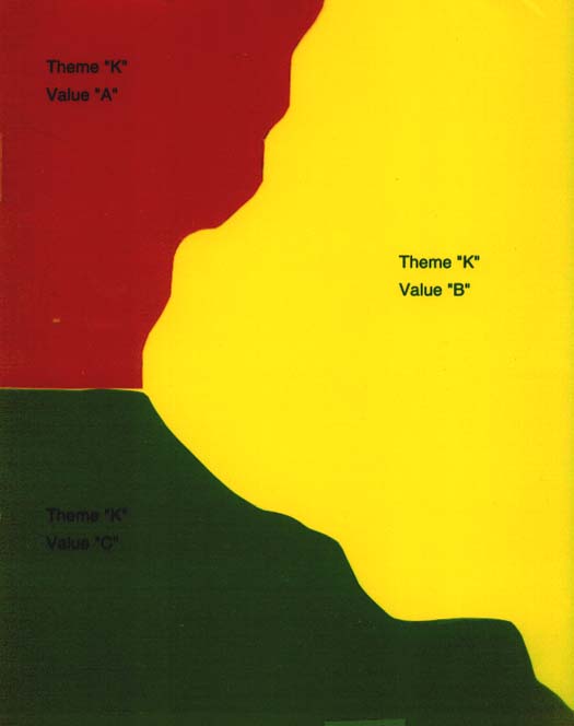
Once probabilities of correctness have been embedded in a dot-raster this information could be used to develop grids or coverages showing those areas that have a minimal level of accuracy. For example suppose a polygon-based coverage named "K" had themes "A", "B", and "C". The tacit assumption made by polygon based GISs is that each theme boundary is a hard and fast line. We know, of course, for the situations we find in nature, that such lines rarely exist, whether we are concerned with forests, streams, flood planes or other naturally occurring phenomena.

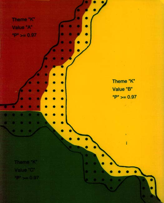
By spatially aggregating those dots whose probabilities were greater than or equal to 0.97 and forming new polygons we can provide a polygon coverage in whose boundaries we can place greater confidence. The areas between the polygons are shown with dots, which all have values of less than 0.97.

such that the cyan areas are polygons where we have confidence in the boundaries and the blue areas represent places in which we are less sure.

Assignment of Dot Values by Infilling

Given the existence of a dot-raster of "dcp" value 2 to the "m", where "m" is greater than 0, approximately three times as many data-carrying dots may be generated by "infilling" the dot-raster. Infilling consists of generating new dots which are precisely between each pair of adjacent active dots in each horizontal row, likewise for adjacent active dots in vertical columns, and in the center of each square formed by a set of four original adjacent active dots.

Active dots of an original dot-raster and an infilled dot-raster are shown below. The new dots are shown by "+" signs:

The result is a dot-raster with a "dcp" of 2 to the "m-1". Each new active dot's "z" value comes from consideration of its neighboring dots. Each "p" value comes (a) from consideration of the "p" values of the neighboring dots, (b) from consideration of the "z" values of neighboring dots, (c) from statistical measures related to the characteristics of the theme being portrayed, and (d) from consideration of the distance between active dots of the original theme.

If more intense infilling were desired (i.e., going from a "dcp" equal to "m," to a "dcp" equal to "m-2" or "m-3"-- which we might call "order 2 infilling" or "order 3 infilling") the DPP infilling procedure described above would not be appropriate (even though using it recursively would result in a database of correct "dcp"). Rather infilling should take place by defining new dots closest to original active dots and repeating this procedure until the proper order of infilling has been achieved.

Assignment of Dot Values by Overlaying

Two dot-rasters that are positionally congruent and which have the same "dcp" may be overlaid. (If the "dcp's" of two dot-rasters "A" and "B" are not equal, and overlaying is desired, one dot-raster might be infilled. Alternatively or additionally, the other dot-raster might be thinned, with, of course, the concomitant loss of data.)

Active dots of a new composite dot-raster may be generated by superimposing (overlaying) two established dot-rasters with identical "dcp's". Given two dot-rasters, say "A" and "B" consisting of thematic or categorical data, for each active dot location the assignment of the value of "z" in the new dot-raster, (say "C"), is based on some function of the corresponding "z" values of "A" and "B". This function could be as simple as the appropriate value in the Cartesian product formed by the possible values of dot-rasters "A" and "B." In general, the value of "z" in dot-raster "C" could be determined by a high-level language program, or by a ProLog or other AI procedure.

The value of "p" for a given dot in "C" represents the joint probability of the correctness of the new value of "z"; it could be the product of the "p" values of the co-located pair of dots in "A" and "B", or the result of a more sophisticated statistical and user-directed process, as indicated by the following.

The actual resulting probability of the overlay of a pair of dots from two dot-rasters may well not simply be the product of the associated values of "p". The resulting value of "p" in the composite dot-raster may depend on many factors, but certainly one might consider the values of "z" in each dot-raster. If one overlays land use and land cover, and the two values are "pasture" and "grass" the probability of correctness might be increased. On the other hand if the values are "pasture" and "pavement" the probability might be decreased. Therefore the software allows the user, for each value in the Cartesian product, to specify an integer "i" in the range [-m to m] such that, for positive "i" the probability "p" is increased above the product of the constituent probabilities; for negative "i" the probability is decreased. For "i" equal to "m", the resulting probability is one; for "i" equal to "-m", the resulting probability is zero. The function is linear. The development of the weighting table is begun with the dpp1 menu.

Suppose we convert the soil suitability coverage that is positionally congruent with the landuse coverage used previously. Our dot-raster (value and probability parts) might look like this:

Overlaying the landuse dot-raster with the soil suitability dot-raster is accomplished with the Intersect menu:

This results in a third dot-raster giving the values (from the Cartesian Product) and the probabilities of correctness, illustrated below:

The lighter the area the lower the probability that the indicated value is correct.

Of course, such an overlay operation decreases the confidence we can place in the values of most locations of the area. The areas (shown below in cyan) in which we are 60% sure that the resultant coverage correctly represents both constituent themes appear below. Dark blue shows areas of less certainty.

Use of the DPP for Point, Line, and Other Data

When using the DPP with point and line data, the active dots are simply those dots used to define the feature; the "dcp" plays no role. That is, every dot is addressable. Thus, using our assumed resolution of 1 cm, points could be delineated within 0.5 cm.

The DPP could store traditional point data by providing the coordinates of the dot closest to the reference point on the object being depicted. The "z" value would simply name the object; the "p" value might indicate spatial (x,y) precision.

Linear data could be stored by simply connecting the relevant dots. The "p" values for each dot used could again indicate spatial(x,y) precision.

It is not hard to envision TIN data, land records data, and data from surveyors in this system.

Favorable Characteristics of the Dot-Probability Paradigm

The author contends that the Dot Probability Paradigm has a number of characteristics that make it attractive as a method of spatial data storage and processing.

1. The DPP has built into it the basis for quality control (QC). Measures for overall coverage accuracy -- whether of input or computed coverages-- would be easy to derive by computation, as would be estimates of accuracy related to particular geographic areas within the coverage and/or particular feature types. And, of course, accuracy measures can displayed visually.
2. Developed and developing statistical and numerical analytic techniques may be applied to the data in the DPP. In particular, many of the techniques used to enhance satellite image data could be applied. Formally, a given DPP dataset could be considered a point sample.
3. The DPP would allow the tool of fuzzy set theory to be applied to spatial data in a straightforward way.
4. The paradigm accommodates both traditional point data and traditional linear data.
5. The re-emergence of cell-based modeling systems as major analytical GIS tools, and their integration with vector based systems, fits well with the raster nature of the DPP.
6. The increasing availability of parallel machines and appropriate algorithms would serve the DPP quite well. DPP spatial overlaying is fundamentally a set of processes -- each concerned with a "more local" geographic area than processes on areas represented by a polygon system -- which maybe conducted in parallel, as no particular sequence is implied.
7. The DPP is highly compatible with remote sensing datasets and with raster-based graphics. Its compatibility with raster I/O devices is obvious.
8. Integer arithmetic may be used to determine the addresses of dots. Such an addressing scheme may be many times faster than those requiring floating point arithmetic. Using a full (32 bit) word for each dimension of the address (for the subscripting value), assuming 31 bits for the number, would provide coverage of an area equivalent to more than one-fifth of the earth's total surface, with dots spaced 1 cm apart; this probably constitutes an adequate tile size at a reasonable resolution for most applications. The values of "p" likewise could be stored as integers, scaled when necessary for use in some computations.
9. Viewed in another way, the DPP could serve as the vehicle for the implementation of the Strabo Technique, as proposed by Dr. Thomas Poiker of Simon Fraser University. Under Strabo -- which has parallels to the Delphi Technique-- experts provide spatially distributed information to which they attach levels of confidence.
10. Overlaying datasets with DPP does not involve the exponential increase in data volume that polygon overlay does. For example, overlaying just a single, simple polygon from each of three layers results in 17 polygons.

Areas for Research

Several issues would have to be addressed before the DPP could become a viable technique in production GISs for spatial data storage and processing. Only a prototype exists based on ArcInfo and ArcView. Further, the DPP could lead to several interesting research projects. A partial list addressing these concerns might include:

1. Theoretical and automated techniques for determining "p" values to be assigned to various types of coverages, and to features within a coverage.
   
2. Reforming dot coverages into polygon coverages, perhaps taking probabilities of accuracy into account and forming polygons indicative of different levels of accuracy.
   
3. Integration of the DPP into existing software packages.
   
4. DPP and fuzzy sets; how can "z" and "p" play a role?
   
5. Using the DPP in measuring heterogeneity; in auto-correlation.
   
6. Developing mechanisms for data compression and use of raster-based storage techniques such as quad trees.
   
7. Exploration of picture enhancement techniques applied to DPP.