Metroscope in Detail
METROSCOPE:
SIMULATING FUTURE URBAN LANDSCAPES AT THE PARCEL LEVEL
Karen Larson
Associate GIS Specialist
Jim Cser
GIS Intern
Sonny Conder
Principal Transportation Planner
Data Resource Center
Metro
conders@metro.dst.or.us
Prepared for the Twentieth Esri International User Conference June 26 – 30, 2000
METROSCOPE:
SIMULATING FUTURE URBAN LANDSCAPES AT THE PARCEL LEVEL
Abstract
Over the last decade National and State requirements have stimulated a vast increase in the sophistication and complexity of integrated land use and transportation models. Along with the increasing economic and computational sophistication of models has been a growth of demands on GIS to simultaneously produce aggregate data while storing and displaying highly disaggregate data. Metro has developed a GIS based tool called Metroscope that works with Metro's real estate and transportation models. Metroscope aggregates parcel based data to a model compatible form, receives aggregated output from the models and converts the modeled output back into parcel format constituting in effect a synthetic future landscape.
Introduction
In response to the policy and forecast demands of managing regional growth, Metro has developed a set of econometric, real estate and transportation models to realistically simulate how markets respond to government growth management and transportation policies. For computational reasons highly iterated transportation and real estate models are presently restricted to a limited number of zones. However, policy and transportation analyses have come to require very detailed data at block level spatial scales. Concomitant with the increasing need for ever finer spatial detail has been a combinatorial explosion in data output. When once we were content with population and employment estimates, we now have hundred's of demographic, employment, real estate, and transportation variables. Given the enormous requirements for data handling, preparation, visualization and accounting, we have used GIS to integrate the various model data flows and locate model zone level output to far more detailed levels of geography. The resultant GIS based system we refer to as Metroscope.
Background of Metro's Modeling Effort
Metro's interest in integrating transportation and land use modeling began initially in 1992 and was and continues to be stimulated by a growing number of Federal, State and local information and compliance requirements. Beginning in the 1990's with Federal legislation such as ISTEA & TEA-21 along with EPA air quality conformity requirements put an increased emphasis on the land use and associated air quality effects of transportation investment. Significantly, at this time there were successful court challenges of MPO transportation plans in California, New York and Illinois based on failure to account for the land use impacts of planned transportation improvements. This litigation further stressed the need to explicitly represent the relationship between land use and transportation within the framework of a consistent, formal simulation model.
Likewise at the State or Oregon and local level new planning requirements demanded information that ultimately must be determined by integrated transportation – land use models; for instance, the maturation of the Urban Growth Boundary (UGB) requirements particularly in the Metro Region. Throughout the 1980’s the UGB amounted to a set of oversized new clothes relative to the growth needs of the region. Only in the early 1990’s did the Metro Region finally began to grow into the boundary. Finally, by the mid to late 1990’s Metro began to grow out of the UGB. State requirements to expand the boundary to maintain a 20 year residential land supply have now precipitated an additional set of questions regarding the interrelationships between housing prices/rents, urban densities, redevelopment and infill rates, travel distances and the share of the economic region’s growth we expect within the UGB. Attempting to verbally unravel such a complex fabric remains completely hopeless. However, integrated transportation – land use models properly formulated are capable of providing estimates of all the above factors for any combination of UGB expansion, zoning capacity and transportation/infrastructure investment policy that might be proposed.
GIS Requirements
Growing model sophistication has placed increasing demands and reliance on the GIS system. Present transportation model development underway at Los Alamos National Laboratories and Portland Metro (TRANSIMS) requires detailed block by block land use and demographic data. In response to these demands Metro has developed a suite of four models embedded in a GIS based system we call Metroscope. As we elaborate below, Metroscope operates as far more than an output visualization tool. Metroscope actually extends the spatial resolution level of the models and incorporates additional spatial information that the models do not use.
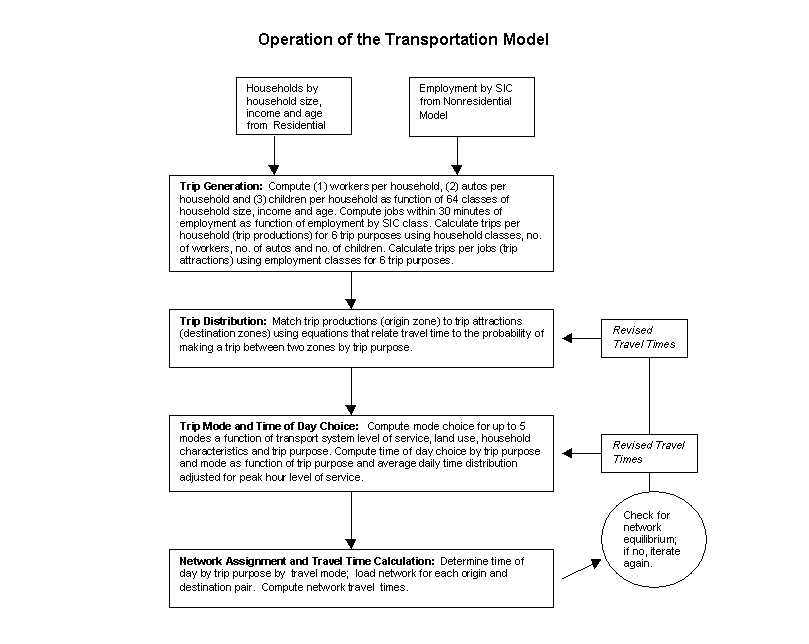
The following schematic shows the flow of information between the various Metroscope modules.
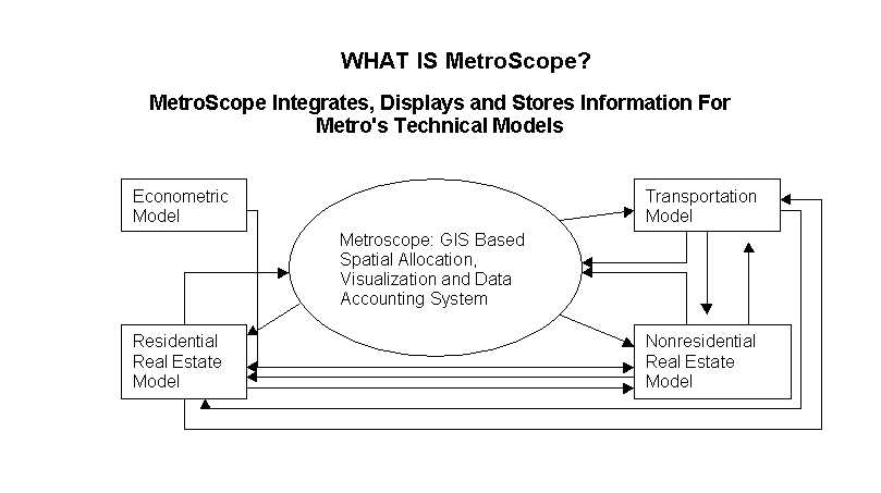
Metroscope Input:
Metro's GIS (RLIS) provides initial condition data to the residential and nonresidential real estate models and the transportation model. These data are aggregated from the parcel level to the appropriate zone or block face system according to the requirements of a particular model. For instance the residential real estate model operates with 400 zones (Census Tracts). The GIS system operating from the parcel level provides the following data to the residential, nonresidential real estate models and the transportation model.
In aggregating parcel level data into zone system data we lose substantial amounts of spatial information such as the distribution of housing by value and urban amenities within the zone. Keep in mind that the modeling system need recover much of that information after the real estate and transportation models have produced their outputs.
Description of Metroscope Components
The following schematics illustrate the information processing and outputs generated within the two real estate models and the transportation model.
Operation of the Nonresidential Real Estate Model
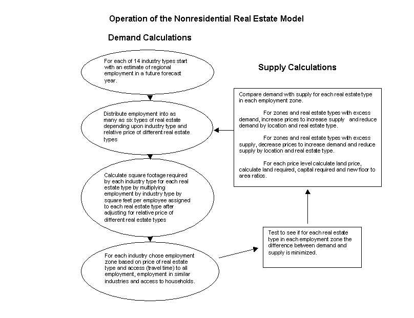
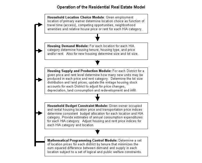
All three of the above models can be considered equilibrium models in the sense that a set of prices or travel times is computed that insure that the various model components are consistent with one another. In turn the individual models share information so that consistency is assured between models. For instance, the residential real estate model uses employment data from the nonresidential model and travel times from the transportation model. By the same token, the nonresidential model uses households from the residential model and travel times from the transportation model. Finally, the transportation model uses household and employment data from both real estate models.
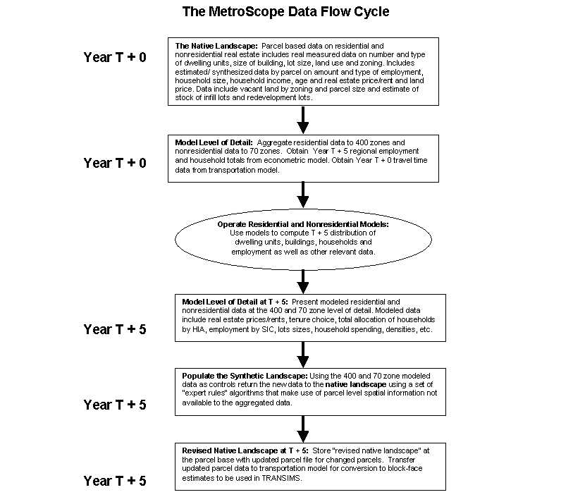
Metroscope in Detail
As noted above the GIS serves several roles in regard to Metroscope operation. These are data accounting, data visualization and mapping model control zone output down to the parcel level. The following schematic illustrates how the GIS moves data back and forth between the parcel based accounting system and the level of geography native to the models and the data visualization system.
As can be noted from the above schematic, the Metroscope approach is to cycle a composite of actual and estimated parcel level data into and out of a modeling process over time. The result is that parcel level data evolve over time as vacant land is developed, areas are redeveloped and populations come and go. Vital to this process is the use of algorithms that allow consistent communication between the parcel level data and the economically powerful but spatially limited operations occurring in the real estate and transportation models. The following Figures and Tables provide a graphic example of how this process works.
Figure One: Year 1999 Actual Parcel Based Data Provide the Metroscope Initial Conditions – Census Tract 12.01 Zoning & Taxlots
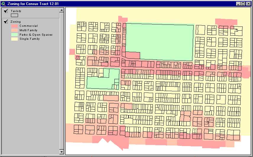
Figure One displays some of the parcel level data that are aggregated to the Census Tract level for use in the real estate models. Table One provides the tabular counterpart to Figure One. In Table One vacant land by parcel size and zoning is aggregated to the Census Tract level. Similarly, housing stock data are extracted from the parcel data and combined with Census data, building permit data and real estate price survey data to yield an estimate of existing housing stock by price/rent category.
Table One: Vacant Land by Parcel Size and Zoning and Housing Stock by Tenure and Price Category Provide Supply Data to the Residential Real Estate Model
|
Census Tract: 12.01 |
||||||||
|
Model Level 1999 Vacant Land Inventory |
Model Level Vintage Housing Inventory |
|||||||
|
Parcel Size |
||||||||
|
Category – Acres |
SFD |
SFA |
MFD |
1990 Census |
1995 Estimate |
|||
|
1000 - 2500 Lot Size Cat. Min-Max Sq. Ft. |
Dwelling Units |
Dwelling Units |
||||||
|
< .5 |
0 |
0 |
0.32 |
Own:0-49.99 |
117 |
0 |
||
|
.5 - .99 |
0 |
0 |
0 |
Own:50-74.99 |
140 |
8 |
||
|
1 - 4.99 |
0 |
0 |
0 |
Own:75-99.99 |
18 |
70 |
||
|
5 - 9.99 |
0 |
0 |
0 |
Own:100-119.99 |
18 |
48 |
||
|
10 - 19.99 |
0 |
0 |
0 |
Own:120-149.99 |
0 |
107 |
||
|
20 plus |
0 |
0 |
0 |
Own:150-174.99 |
0 |
81 |
||
|
2500 - 5000 Lot Size Cat. Min-Max Sq.Ft. |
Own:175-199.9 |
0 |
23 |
|||||
|
< .5 |
0 |
0.31 |
0.72 |
Own:200+ |
0 |
25 |
||
|
.5 - .99 |
0 |
0 |
0 |
Total: |
293 |
362 |
||
|
1 - 4.99 |
0 |
0 |
0 |
|||||
|
5 - 9.99 |
0 |
0 |
0 |
Rent:0-199 |
176 |
74 |
||
|
10 - 19.99 |
0 |
0 |
0 |
Rent:200-299 |
433 |
128 |
||
|
20 plus |
0 |
0 |
0 |
Rent:300-399 |
939 |
361 |
||
|
5000 - 7000 Lot Size Cat. Min-Max Sq. Ft. |
Rent:400-499 |
395 |
629 |
|||||
|
< .5 |
0.23 |
0 |
0 |
Rent:500-599 |
73 |
645 |
||
|
.5 - .99 |
0 |
0 |
0 |
Rent:600-749 |
39 |
331 |
||
|
1 - 4.99 |
0 |
0 |
0 |
Rent:750-999 |
0 |
72 |
||
|
5 - 9.99 |
0 |
0 |
0 |
Rent:1000 |
0 |
8 |
||
|
10 - 19.99 |
0 |
0 |
0 |
Total: |
2055 |
2250 |
||
|
20 plus |
0 |
0 |
0 |
|||||
Table One presents the vacant land data displayed spatially in Figure One in tabular form arrayed and aggregated for use in the residential real estate model. Table One also contains data on the existing dwelling units displayed in Figure One. Here too, the data have been converted from their spatial context to the aggregated tabular context necessary for use in the modeling framework.
From Table One we note that our inner city census tract, 12.01 contains very little vacant land about 1 acre for multi-family and ˝ acre for single-family. All of the vacant land occurs on parcels of less than ˝ acre. The existing residential real estate data indicates about 300 owner occupied and 2000 renter occupied units exist in the tract as of 1995. Price/rent data indicate that the stock has appreciated in price between 1990 and 95 but was generally still low in value. The residential model automatically adjusts capacity to account for infill and redevelopment. Areas with little vacant land, relatively low values for existing stock and high demand will generate 10 – 20 units of infill and redevelopment for every unit developed on vacant land. Conversely, areas with ample vacant land and high values for existing stock will experience 1 – 2 units of infill and redevelopment for every 10 – 15 units developed on vacant land.
Figure Two displays at the 400 zone level some of the year 2000 output of the residential real estate model. In this instance we are displaying the tenure choice (percent owner) by census tract of one person households, age 25 - 54 years with an income between $29,000 and $43,000. (Keep in mind we have the option of show 64 combinations of household size, income and age for up to 20 variables.)
Figure Two: Using Initial Condition Land Use Data, Travel Times and Regional Growth Data the Residential Model Allocates Households and Real Estate
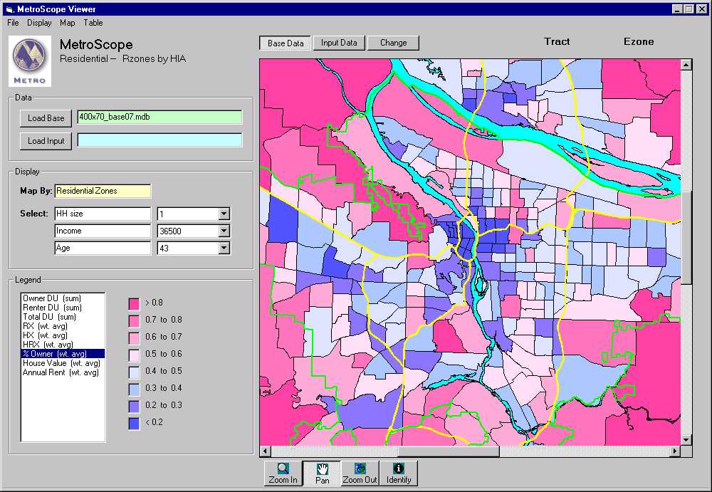
Figure Two shows the pattern for the entire region of where a particular household size, income and age class chooses to locate and whether they are owners or renters. Should we choose, we could show the same data or any of 64 HIA classes or show a summary for all classes.
Table Two summarizes the census tract aggregate data showing the updated year 2000 housing stock by price/rent category. Notable is that despite almost no vacant land the housing stock has increased over 100 units due mainly to infill and redevelopment. Significantly, owner occupied has increased, renter occupied has decreased and overall prices and rents have continued to increase.
Table 2: Year 2000 Housing Stock Increases Over the 95 Level in Number and Value but Renter Decreases Slightly
|
Census Tract: 12.01 |
|
|
Model Level Housing Output |
|
|
2000 Estimate |
|
|
Dwelling Units |
|
|
Own:0-49.99 |
0 |
|
Own:50-74.99 |
5 |
|
Own:75-99.99 |
100 |
|
Own:100-119.99 |
117 |
|
Own:120-149.99 |
98 |
|
Own:150-174.99 |
48 |
|
Own:175-199.9 |
100 |
|
Own:200+ |
21 |
|
Total: |
489 |
|
Rent:0-199 |
0 |
|
Rent:200-299 |
0 |
|
Rent:300-399 |
559 |
|
Rent:400-499 |
633 |
|
Rent:500-599 |
333 |
|
Rent:600-749 |
414 |
|
Rent:750-999 |
286 |
|
Rent:1000 |
0 |
|
Total: |
2225 |
In Figure Two census tract 12.01 is simply a blue patch on the map display. Likewise, in Table Two the data are highly aggregated and totally bereft on any spatial context below the census tract boundaries.
Figure Three presents the aggregate data in Figure Two after it has been processed back to the parcel level. In this case we have retained owner/renter choice and 4 income classes. Conceptually, it is possible to allocate owner/renter choice over all 64 classes of household size, income and age for a total of 128 different variations. However, such an extremely busy display would muddle far more than it would clarify. Rather, we have chosen to limit the display to 8 classes.
Figure Three: Residential Model Ouput for Census Tract 12.01 is Allocated Back to the Parcel Level Using Parcel Based Spatial Information
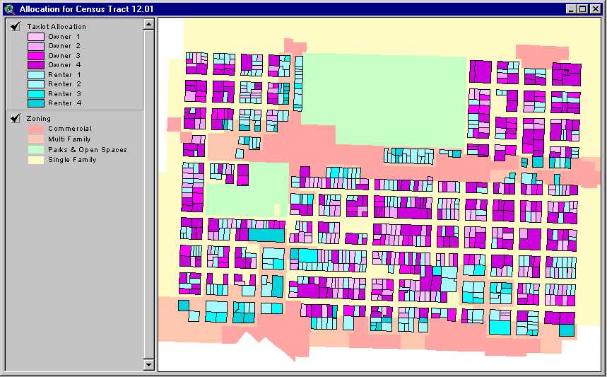
Figure Three provides far more spatial and socio-economic detail than was available in the regional level data. In Figure three we note that roughly half the area is taken by owner occupied dwellings though they comprise less than 20% of the households. This underscores the much higher densities of renter occupied structures. Similarly, owners are predominately from the middle and high income groups while renters represent low and moderate income groups. All of the modeled data though produced on an aggregated basis, has now been disaggregated back to the parcel level to create a synthetic landscape.
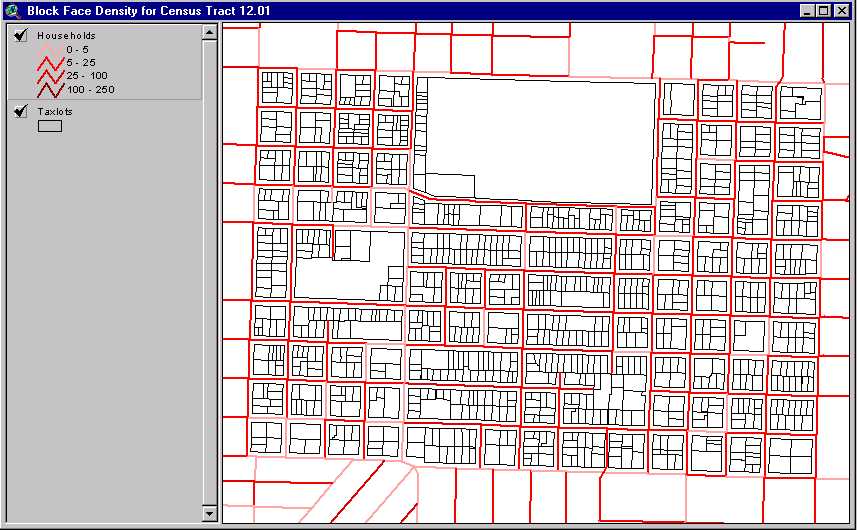
Figure Four displays the final step in creating a synthetic future landscape compatible with the latest transportation models (TRANSIMS). These maps are produced after the parcel level data displayed in Figure Three are passed over to the transportation model. The parcel level density information implicit in Figure Three in then converted to "block face" household densities to be used for generating trip making patterns in the transportation model.
Figure Four: Parcel Level Household Allocation is Converted to Block Face Household Density for Use in TRANSIMS Modeling
Conclusion
Over the past several years both National and State requirements have placed ever greater demands on the technical aspects of modeling land use and transportation. At one end the increasing requirements for integration of land use and transportation in an economically realistic and consistent framework has lead to highly iterative systems of hundreds of simultaneous equations. Necessarily for computational and theoretical reasons these requirements have lead to use of aggregated data in fairly large zones. At the other end are the requirements to make the maximum use of the detailed spatial and nonspatial information that GIS has made available to us. In this paper we have demonstrated a system whereby streams of parcel level data are aggregated and converted to a model useable format. In turn once the data are processed in the models we reverse the process so that the spatial and other omitted data are returned to the system on an estimated or "synthesized" basis. In addition the data streams generated by the models may be visualized using GIS at several levels of aggregation depending on the type of data and the interests of the user. Model data output consistently returned to the parcel level also provides the initial conditions for use in the next modeling period.
References:
Friesen, P. & Lydon, B. Modeling Land Use Change: Using GRID to Develop Scenarios for Colorado Springs' Comprehensive Plan, Esri 1999 Proceedings Paper 222, 12 pages.
Mitchell, A. ; Population and Demand Allocation Using Polygon Overlay Techniques, Esri 1999 Proceedings, Paper 552, 10 pages.
Waddell, P. ; Residential Property Values in a Multinodal Urban Area: New Evidence on the Implicit Price of Location, Journal of Real Estate Finance and Economics; (1993), pp 117 – 141
Waddell, P.; Vibhooti, S.; Employment Dynamics, Spatial Restructuring and the Business Cycle, Geographical Analysis, (1993), pp 35 – 52.
Abraham, J.;Hunt, J.; Policy Analysis Using the Sacramento Meplan Land Use Transportation Interaction Model, (1999) TRB Presentation, 21 pages.
Anas, A.; Rong, X.; Congestion, Land Use, and Jobs Dispersion: a General Equilibrium Model, Journal of Urban Economics, (1999), pp. 451 – 473.
McMillen D.; McDonald, J. Suburban Subcenters and Employment Density in Metropolitan Chicago, Journal of Urban Economics, (1998), pp 157 – 180
Wheaton, W.; The Cyclic Behavior of the National Office Market, AREUEA Journal, (1987), pp 281 – 299.
Wheaton, W.; Torto, R.; An Investment Model of the Demand and Supply for Industrial Real Estate, AREUEA Journal, (1990), pp. 530 – 547
Thompson, R.; Industrial Employment Densities, Journal of Real Estate Research,(1997), pp 309 – 319.
Hakfoort, J.; Lie, R.; Office Space per Worker: Evidence from Four European Markets, Journal of Real Estate Research, pp 183 – 196
Clapp, J.; Pollakowski, H.; Lynford, L. Intrametropolitan Location and Office Market Dynamics, AREUEA Journal, (1992), pp. 229 – 257.
Colwell, P.; Munneke, H.; Trefzger, J.; Chicago's Office Market: Price Indices, Location and Time; Real Estate Economics, (1998), pp 83- 106.
Benjamin, J.; Jud G.;Winkler, D.; A Simultaneous Model and Empirical Test of the Demand and Supply of Retail Space, Journal of Real Estate Research, (1998), pp 1 – 13.
Tsolacos, S.; Keogh G.; McGough, T,; Modeling use, investment, and development in the British office market, Environment and Planning A,(1998), pp 1409 – 1427.
Buttimer, R.; Rutherford, R.; Witten, R., Industrial Warehouse Rent Determinants in the Dallas/Fort Worth Area, Journal of Real Estate Research, (1997), pp 47 – 55.
Okoruwa, A.; Nourse, H.; Terza, J.; Estimating Sales for Retail Centers: An Application of the Poisson Gravity Model, Journal of Real Estate Research, (1994), pp. 85 – 97.
DiPasquale, D.; Wheaton,W.; Housing Market Dynamics and the Future of Housing Prices; Journal of Urban Economics; (1994), pp 1 - 27.
Randolph, W.; Estimation of Housing Depreciation: Short-Term Quality Change and Long -Term Vintage Effects, Journal of Urban Economics; (1988), pp 162 - 178.
Rubin, J.;Seneca, J.; Density Bonuses, Exactions, and the Supply of Affordable Housing; Journal of Urban Economics; (1991), pp 208 - 223.
Brueckner, J.; Growth Controls and Land Values in an Open City; Land Economics; (1990), pp 237 - 248.
Palmquist, R.; Valuing Localized Externalities, Journal of Urban Economics; (1992), pp 59 - 68.
Malpezzi, S.; Ozanne, L.; Thibodeau, T.; Microeconomic Estimates of Housing Depreciation; Land Economics; (1987); pp 372 - 385.
Harmon, O.; The Income Elasticity of Demand for Single-Family Owner-Occupied Housing: An Empirical Reconciliation; Journal of Urban Economics; (1988), pp 173 - 185.
Glennon, D.; Estimating the Income, Price, and Interest Elasticities of Housing Demand; Journal of Urban Economics; (1989), pp 219 - 229.
McGibany, J.; The Effect of Property Tax Rate Differentials on Single-Family Housing Starts in Wisconsin; Journal of Regional Science; 1978 - 1989; (1991), pp 347 - 359.
Singell, L.; Lillydahl, J.; An Empirical Examination of the Effect of Impact Fees on the Housing Market; Land Economics; (1990), pp. 82 - 92.
Herrin, W.; Kern, C.; Testing the Standard Urban Model of Residential Choice: An Implicit Markets Approach; Journal of Urban Economics; (1992), pp 145 - 163.
Cobb, S.; The Impact of Site Characteristics on Housing Cost Estimates; Journal of Urban Economics; (1984), pp 26 - 45.
Vaillancourt,F.; Monty, L.; The Effect of Agricultural Zoning on Land Prices, Quebec, 1975 - 1981; Land Economics; (1985), pp 36 - 42.
Dunford, R.; Marti, C.; Mittelhammer, R.; A Case Study of Rural Land Prices at the Urban Fringe Including Subjective Buyer Expectations; Land Economics; (1985), pp 11 - 16.
Anas, A.; Chu, C.; Discrete Choice Models and the Housing Price and Travel To Work Elasticities of Location Demand; Journal of Urban Economics; (1984), pp 107 - 123.
Munneke, H.; Redevelopment Decisions for Commercial and Industrial Properties; Journal of Urban Economics; (1996), pp 229 - 253.
Stover, M.; Specification Error in the Estimation of the Elasticity of Substitution; Annals of Regional Science; (1990), pp 122 - 131.
Lapointe, A.; Desrosiers, J.; Modeling Residential Choice; Journal of Regional Science; (1986), pp 549 - 566.
Knapp, G.; The Price Effects of Urban Growth Boundaries in Metropolitan Portland, Oregon; Land Economics; (1985), pp 26 - 35.
Rosenthal, S.; Helsley, R.; Redevelopment and the Urban Land Price Gradient; Journal of Urban Economics; (1994), pp 182 - 200.
McAndrews, J.; Voith, R.; Can Regionalization of Local Public Services Increase a Region’s Wealth?; Journal of Regional Science; (1993), pp 279 - 301.
Stover, M.; The Role of Infrastructure in the Supply of Housing; Journal of Regional Science; (1987), pp 255 - 267.
McDonald, J.; Capital-Land Substitution in Urban Housing: A Survey of Empirical Estimates; Journal of Urban Economics; (1981), pp 190 - 211.
Jackson, J.; Johnson, R.; Kaserman, D.; The Measurement of Land Prices and the Elasticity of Substitution in Housing Production; Journal of Urban Economics; (1984), pp 1 - 12.
Somerville, C.; Analyzing Construction Costs: Builder Behavior and Sub-Contractor Reputation in Homebuilding; (unpublished UBC 1994), 32 pages.
Shields, M.; Time, Hedonic Migration, and Household Production, Journal of Regional Science; (1995), pp 117 - 134.
Cervero, R.; Wu, K.; Subcentering and Commuting: Evidence from the San Francisco Bay Area; (Working Paper no. 668, U. of California, Berkeley, 1996), 31 pages.
Burchell, R.; Listokin, D.; Land, Infrastructure, Housing Costs and Fiscal Impacts Associated with Growth: The Literature on the Impacts of Sprawl versus Managed Growth; (Lincoln Institute of Land Policy Research Papers, 1995), 25 pages.
Knapp, G.; The Determinants of Metropolitan Property Values: Implications for Regional Planning; (Metro, 1996), 51 pages.
City of Portland Auditor; Multnomah County Auditor; Housing: Clarify Priorities, Consolidate Efforts, Add Accountability; (City of Portland, Audit Services Division, 1997), 64 pages.
Metro; Housing Needs Analysis - Technical Appendix 1; (Metro Growth Management Services Department, 1997), 139 pages.
Sonny D. Conder
Principal Transportation Planner
Metro Data Resource Center
600 NE Grand
Portland, OR 97232
Tel (503) 797 – 1592
Fax (503) 797 – 1909
E-Mail Conders@metro.dst.or.us