
Theodore Shannon1, John W. Labadie2, Marc Baldo3, Roger Larson4
Abstract:
The U.S. Bureau of Reclamation has completed a major study that documents the economic, environmental and social impacts of annually delivering up to 1,427,000 acre-feet as flow augmentation for various fishery species that live and pass through the Lower Snake River, Idaho. The generalized river basin network flow model MODSIM was applied by Reclamation for this study due primarily to its unique capability of integrating the physical, hydrologic, and administrative aspects of evaluating the impacts of various flow augmentation scenarios. MODSIM includes the capability of incorporating spatially distributed stream-aquifer response coefficients generated from the USGS MODFLOW model. GIS plays a major role in synthesizing these spatially distributed response coefficients for inclusion into MODSIM. This paper presents prototype software which provides a metadata framework for linking GIS coverages with the procedural MODSIM river basin network flow model, with application to the Lower Snake River flow augmentation study.
Concerns for the propagation of endangered salmon and steelhead that live and migrate through the Lower Snake River of Idaho have prompted discussion for increasing instream flows using U.S. Bureau of Reclamation (USBR) projects. The USBR has completed a major study at the request of the U.S. Army Corps of Engineers that documents the economic, environmental and social impacts of annually delivering an additional 1,000,000 acre-feet of flow augmentation (USBR, 1999). Reclamation storage is presently used for irrigation water supply, M&I water supply, flood control, hydroelectric generation, resident fish and wildlife considerations, reservoir and instream recreation, and meeting Native American water rights obligations.
Several alternatives for improving fish habitat are being considered, including purchasing water from irrigators, reservoir operational changes, dam modification, and breaching four hydroelectric dams on the Lower Snake River. This large instream flow increase in a complex and already taxed basin has required the need for modeling that considers multidisciplinary issues as well as hydrologic analysis. The generalized river basin network flow model MODSIM, developed at Colorado State University (Fredericks, et al., 1998), was applied by Reclamation for the above mentioned study due primarily to its unique capability of integrating the physical, hydrologic, and administrative aspects for evaluating the impacts of various flow augmentation scenarios. MODSIM allows the model user to determine impacts on physical system features, while providing water rights and storage accounting information in an integrated manner.
This paper describes a GIS application, programmed in Visual C++ using MapObjects, which extends the ability of MODSIM to access and utilize spatial data. An application is described here where arbitrary ground-water model cells can be grouped to calculate steady-state response functions for reaches of the eastern Snake River in Idaho. These spatially distributed response coefficients are then transferred into MODSIM.
River basin network flow models provide an efficient means of simulating large-scale, complex water resource systems in a fully integrated manner. MODSIM represents a decision support system that integrates a powerful graphical user interface (GUI) and spatial data base management system with a generalized river basin network flow model. The network model employs a state-of-the-art network optimization algorithm for simultaneously assuring that water is allocated according to physical, hydrological, and institutional aspects of river basin management, including stream-aquifer interactions (Fredericks, et al. 1998). Although MODSIM is an optimization model, the attempt is to employ optimization methods as an efficient mechanism for performing simulation. The minimum cost network flow problem is solved sequentially over time as:
subject to:


where A is the set of all arcs or links in the network; N is the set of all nodes; Oi is the set of all links originating at node i (i.e., outflow links); Ii is the set of all links terminating at node i (i.e., inflow links); qR is the integer valued flow rate in link R ; cR are the costs, weighting factors, or priorities per unit of flow rate in link R ; lR is the lower bound on flow in link R; and uR is the upper bound on flow in link R.
The network flow optimization problem is solved using an efficient dual coordinate ascent procedure based on Lagrangian relaxation (Bertsekas and Tseng, 1994). Eq. 2 guarantees satisfaction of hydrologic mass balance throughout the network. Eq. 3 maintains specified flow limits for all links, as well as providing a means of accounting for lagged return flows, stream depletions, and channel losses
Consumptive Demands and Instream Flow Requirements
MODSIM automatically creates accounting links which originate at each demand node and accumulate at a single accounting demand node D. Demands are assigned as upper bounds on flows in these links, with lower bounds set at zero. This allows shortages to occur if water supply is limited and the demand is of junior priority. Demands may be defined as historical diversions, decreed water right amounts, predicted agricultural demands based on consumptive use calculations (performed outside the model), or projected municipal and industrial demands. Multiple links may be connected to a demand, representing several decreed water rights with different priorities. The maximum possible total delivery is dictated by the lower of the sum of the decreed water rights, the demand assigned to the node, and the capacity of the diversion structure or structures delivering the flow.
MODSIM also provides for demands for water which are not terminal; i.e., instream flow demands which flow-through the demand node and remain in the network for possible downstream diversion. The flow-through demand operates by iteratively removing flow as a demand from the network, but then replacing the flow at one or more specified (usually the next downstream) node(s), which essentially corresponds to demands with 100% return flow which is unlagged. Flow-through demands are applied to instream flow uses for navigation, water pollution control, fish and wildlife maintenance and recreation which can be assigned water right decree priorities like any other demand. Flow-through demands are also useful for augmentation plans, exchanges between basin water users, and development of reservoir release operating rules.
The mathematical flow equation for general two dimensional flow in an unconfined aquifer, assuming variation in saturated thickness is small, is written as (Willis and Yeh, 1987):

where T is transmissivity (L2t-1) = Kb, K is hydraulic conductivity (Lt-1), b is saturated thickness (L); h is potentiometric head (L); Q is net groundwater withdrawal per unit area (Lt-1); S is storage coefficient (L-1); and t is time (t).
Eq. 4 can be solved using finite difference or finite element numerical methods (Willis and Yeh, 1987) using discrete points or grids for calculating finite differences in potentiometric head, resulting in systems of linear algebraic equations. Maurer (1986) used the USGS modular three-dimensional finite-difference groundwater flow model MODFLOW (McDonald and Harbaugh, 1988) to simulate the effects of groundwater development in the Carson Valley, Nevada.
Since the governing groundwater flow equation (4) is linear and time invariant, linear system theory can be applied via the principle of superposition (Bear, 1979), allowing individual excitation events to be calculated independently and their responses linearly combined. Applying linear system theory to the groundwater flow equation allows use of Green's function to solve the resulting non-homogeneous boundary value problem (Maddock, 1972). Response of the groundwater system due to external excitations such as pumping, recharge, or infiltration at any point in space and time can be expressed as a set of unit coefficients independent of the magnitude of the excitation.
Morel-Seytoux and Daly (1975) developed a finite difference model to generate any aquifer response as an explicit function of pumping rates, which they referred to as a discrete kernel generator. The discrete kernel method has been utilized extensively as a tool for solving complex groundwater management problems (Illangasekare and Morel-Seytoux, 1986; Illangasekare and Brannon, 1987). Maddock and Lacher (1991) developed MODRSP as a modified version of MODFLOW for calculating kernel or response functions for stream-aquifer interactions. MODRSP is an appropriate numerical model for determining response function coefficients since it allows modeling of a multi-aquifer groundwater flow system as a linear system with irregularly shaped areal boundaries and non-homogeneous transmissivity and storativity. Spatially distributed stream-aquifer response coefficients generated using MODRSP can be used to allocate groundwater return/depletion flows to multiple return/depletion flow node locations anywhere in the river basin network.
The stream-aquifer module within MODSIM allows consideration of reservoir seepage, irrigation infiltration, pumping, channel losses, return flows, river depletion due to pumping, and aquifer storage. For demand node i and any current time period considered, the total return flow IRFik from previous and current time periods due to groundwater recharge is calculated as:

where I_{i tau} is the infiltration rate at node i, period J , and *i,k-J+1 is the discrete kernel coefficient defined for node i, period k-J+1. The discrete kernel coefficients are calculated internally in MODSIM using either the Glover equations or the SDF method, or they can be precalculated externally by a model such as MODRSP and then read into MODSIM as an external data file. In effect, the use of precalculated discrete kernel response coefficients essentially represents the selected groundwater model, but without the need to explicitly run the groundwater model during MODSIM calculations, resulting in considerable savings in computer time.
Physical features such as reservoirs, river reaches, diversions, river gages, etc, are represented on the MODSIM GUI canvas as a network of nodes and links. Nodes may act as reservoirs, surface inflow locations, irrigation demands, municipal demands, groundwater return locations, and minimum stream flow requirements. Links may limit flow, define water rights, or define a connection to storage ownership. The GUI allows the user to enter geo-referenced data associated with objects in the network through a series of spreadsheets. The Snake River network pictured here (figure 1) has 420 nodes and 1,300 links, with an additional 1,000 accounting links to form a fully circulating network.

Figure 1. MODSIM Snake River Network
In the zoomed diagram, the Palisades Reservoir node is shown (figure 2), with its reservoir rule curves for dry through wet years. Each month's target is calculated utilizing forecasted basin inflows and current reservoir contents to determine the current operating rule.

Figure 2. Palisades Reservoir Node from MODSIM
Palisades reservoir is modeled as a single reservoir for evaporation and power calculation, but for reservoir accounting purposes, two account reservoirs have been added. Pal_1&2 reservoir accounts for available water for ownership links, and Pal_PowH reservoir represents the minimum reservoir pool for power generation and operation. The MODSIM reservoir accounting module tracks the amount accrued to each account reservoir, calculates the amount available for each ownership link, and updates the account balances based on evaporation or flood control releases.
The Snake River Plain Aquifer Model (SRPAM) covers the eastern portion of the Snake River Plain (Johnson and Cosgrove, 1999). The model grid consists of 1,083 cells ordered in 63 columns and 48 rows (figure 3). Each raster cell is 25 km2 in area and contains one unconfined aquifer layer. The grid is oriented to run parallel to the plain axis, with the north-south oriented 21o counter clockwise. The grid cells have been partitioned by Johnson and Cosgrove into twenty hydraulically similar regions. The fifty one Snake River cells have been aggregated into six reaches: from Ashton to Lorenzo in the north-east; Heise to Lorenzo; Lorenzo to Lewisville; Shelley to Neeley; Neeley to Minidoka; and Milner to King Hill in the south-west.

Figure 3. SRPAM Model Grid Cells. Source: Johnson and Cosgrove, 1999.
The SRPAM model was updated by Johnson and others to incorporate MODRSP model code. MODRSP uses the finite-difference ground-water model, MODFLOW, to stress an individual grid cell and determines the unit stress on a river reach cell. This effect, a response ratio, describes the proportional change in surface water flow resulting from ground-water extraction or recharge. Johnson and Cosgrove computed response functions for each grid cell on the six river reaches and for 1,200 monthly time steps. The resulting Microsoft Access database consisted of nearly 1.3 million records, with each record containing six river reach response ratios for a given cell and time step. To enhance later queries that compute aggregate response ratios, all of the record fields were indexed. This increased the final size of the database from 70 to 166 megabytes.
The integrated development environment selected for this project is Microsoft Visual C++ 6.0 for the Windows 9x/NT operating systems. Since MODSIM is coded in C++, programming this application in the same language allows for static linkages that embed GIS within the model. This tight integration provides refined and controlled program flow, such as synchronous events, and merging of traditional algorithmic modeling code with spatial databases. The MODSIM model is itself still evolving to meet new challenges; statically linking to MODSIM will ideally minimize maintenance requirements when the model code is upgraded. Mixed language programming, such as writing the GIS interface in Visual BASIC and statically or dynamically linking to the C++ code, is also possible. However, the introduction of intermediate steps in maintaining dynamic link libraries or static object files and having programming staff knowledgeable in multiple languages caused single language development to be favored.
Currently, MapObjects 2 is the selected GIS software component. Based on functionality descriptions from current product literature, MapObjects LT 2, when released, may replace this. While most programming samples for MapObjects are provided in Visual BASIC, the components are almost as easily accessed with C++. Microsoft Access formatted databases and ActiveX Data Objects (ADO) are utilized for database support, allowing structured query language in accessing a variety of data formats including shapefiles.
Integration of GIS with procedural models should be a further step in the trend of generalized modeling tools. First, geographic information systems involve information management as well as spatial functionality. Second, spatial data is often collected and used for purposes other than the requirements of a given model, which makes data reformatting more difficult and lessens the value of spatial data for other applications. Metadata is used to allow the application to search for specific information, which may be located in one or more geodatasets (Rouke, 1998).
Application of metadata to shapefiles involves the creation of a separate Access database that contains two classes of data: dictionaries and metadata. A dictionary defines metadata fields for the software; end users may add or modify the definitions as needed. The main dictionary, the Attributes Dictionary, lists the available attributes that can be applied to shapes and database fields. Examples of attributes include "Canal", "Diversion Structure", and "Irrigation Demand". Each attribute definition further specifies the type of data that it can be applied to (e.g., point coverages only, both line and polygon coverages, or numeric data only).
The Units Dictionary lists the available measurement units. A unit is defined by a name; length, mass, and time dimensions; and information needed to convert the given unit into a default unit set for computations. Stream flow in cubic feet per second would have a length dimension of three, and a time dimension of negative one; it may also have conversion factors for m3 s-1. The available units for a given data set are restricted by the selected attribute. A "Canal" attribute might limit the units to those of linear measure only; "Irrigation Demand" might include both unitless dimensions for point coverages, such as wells, and also area measurements for polygon coverages, such as agricultural fields.
The Role Dictionary defines available roles that data can have in the MODSIM model. This dictionary is separate from the attributes dictionary, as various basin objects can have different roles depending on the scenario. A well may in one case extract ground-water, and in another be a recharge point. A role definition contains a descriptive name and a role type identification number that describes data use to the model. As the role identification number is coded within the application itself, expanding this dictionary requires upgrading the software code. This still provides a framework for creating new modeling objectives for spatial data. Similar to the units dictionary, selecting a given attribute will limit the available roles that data can have in the model. For example, an "Irrigation Demand" can not take on roles involving water storage.
While dictionaries provide descriptions of the metadata, related tables are used to actually store metadata for each geodataset. When a new coverage is introduced to the software, an identification number is assigned to the path and filename to uniquely identify it. A metadata record is created to which this file identification number is linked. The end user may then select an attribute for a given field from a pull-down list populated from the Attributes Dictionary: the corresponding attribute identification number is linked to the metadata record. The selected attribute will populate the units and role pull-down lists from their respective dictionaries, and the attributes from these lists are then linked to the metadata record.
A coverage was created which geo-references the response ratios contained in an Access database. A query was developed which assigns column, row, and grid cell identification number from the database to an ASCII raster grid file. The grid was translated and converted to a polygon coverage using ArcView 3.2. It was then projected into Idaho Transverse Mercator (IDTM) for use with other coverages obtained from the Idaho Geographic Information Center. This polygon coverage was introduced to the application, which then prompted for attribute metadata (figure 4). The shape field of the coverage was assigned an attribute of "Hydrological Unit", the units of "Area (m^2)", and the role of "Model Grid Cell". The grid cell identification field of the coverage was assigned "Identification Number", "(no units set)", and "Grid Identification Number" respectively.
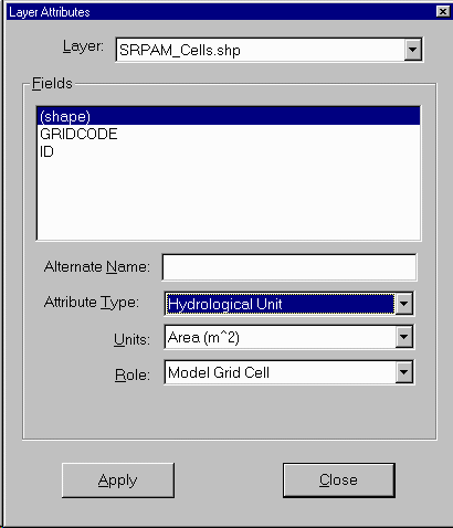
Figure 4. User Interface for Setting Metadata Attributes
To select grid cells from the coverage, the end user activates the "Response Cells" tool (figure 5). The application searches the available map layers for shapes having the role of "Model Grid Cell". The layers meeting this criterion are displayed in a pull-down list. The user than selects the coverage to use (if there is more than one) and may modify output options for the operation. The ActiveX Data Objects are used to create a fabricated database, a dynamic database constructed in random access memory that acts similar to disk-based databases. The fabricated database is used to store intermediate information, in this case the identification numbers of selected model grid cells.
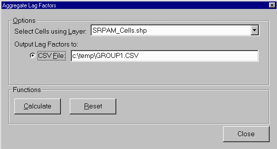
Figure 5. User Interface for the Response Function Tool
When the user points and clicks on a grid cell, or rubber bands a group of cells, the application conducts a spatial search to locate shapes within the selected extent. The field of the selected records containing the grid identification number is found via a metadata search. This data is then added to the fabricated dataset (cell selection), or removed if the cell was previously selected (cell deselection). The process continues, with the user selecting additional cells from the same or a different layer (figure 6).
When the user selects the "Calculate" function, two structured query language (SQL) statements are created from the fabricated dataset. The first SQL statement performs an aggregate counting function, which returns a dataset containing the number of records in each reach and time step. The second SQL statement returns an ordered dataset containing the individual response ratios for a reach and corresponding time steps. Using the first recordset, an index can be calculated which returns the median response ratios from the second dataset. The median ratios are then recorded to an output file for each reach and time step. When the operation is complete, the user can add additional cells to the fabricated recordset or can clear the set by selecting the "Reset" function.
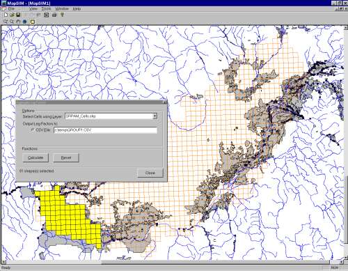
Figure 6. Selecting sample cells from the grid layer
Johnson and Cosgrove (1999) partitioned the grid cells into twenty zones based on similar response to the six Snake River reaches of the SPRAM model. Median response ratios were determined for each zone and river reach. The same zones were selected in the application. Comparisons between the published and derived values are presented in figure 7.

Figure 7. Comparisons of Published Steady State Response Ratios and Application Results
MODSIM scenarios included no flow augmentation (NoAug), the current augmentation of 427,000 acre-feet (427), and an increased instream flow of 1,427,000 acre-feet. There were further two alternatives for obtaining the larger instream flow: from reservoir drawdown (1427r) or from irrigation shortages (1427i). Examples of simulation results are shown in Figures 8 and 9. Figure 8 summarizes annual irrigation shortages in the Snake River Basin for the four studies as a duration curve. Figure 9 shows the deep reservoir drafts that would occur at Cascade Reservoir during the summer recreation period under implementation of the added flow augmentation proposals.

Figure 8. Annual Irrigation Shortage. Source: Larson and Spinazola, 2000.

Figure 9. Deep reservoir drafts - Cascade Reservoir. Source: Larson and Spinazola, 2000.
A prototype software program was presented which represents an initial step toward integrating GIS and a procedural model. The information management framework of the application uses metadata to define how spatial data is used in the model, enhancing data use between model scenarios and different GIS applications. Future work on this project will focus on importing response functions and extracting river basin topology from geodatasets into the MODSIM model.
This project is being funded by the U.S. Bureau of Reclamation.
1 Ted Shannon. Graduate Research Assistant, Dept. of Civil Engineering, Colorado State University, Fort Collins CO 80523
Telephone: (970) - 491 - 5387
Email: tshannon@engr.colostate.edu
2 John W. Labadie. Professor, Dept. of Civil Engineering, Colorado State University, Fort Collins CO 80523
Telephone: (970) - 491 - 6898
Email: labadie@engr.colostate.edu
3 Marc Baldo. Research Associate, Dept. of Civil Engineering, Colorado State University, Fort Collins CO 80523
4 Rodger Larson. Hydraulic Engineer. Bureau of Reclamation, 1150 N. Curtis, Boise ID 83706-1234
Telephone: (208) - 378 - 5274