The utility of current geological maps is limited by the lack of tools to quantitatively summarize and analyze map data. This research created Avenue scripts for ARCVIEW that allow the objective analysis of arcuate geologic map features. The scripts break arcs representing fault traces, fold axes, and geological contacts into line segments whose orientations can be summarized by vector mean calculations and represented as rose diagrams of line trends. This information can then be used to determine the angular relationships between different types of geological data and to test geological hypotheses. These methods were used to test whether the Rocky Mountains in Wyoming, Colorado and New Mexico formed due to multiple stages and directions of compression during the Laramide Orogeny (70-40 Ma). Fault and fold orientations systematically change with latitude from New Mexico to Wyoming, indicating that observations from one location may not be valid elsewhere in the Rocky Mountains. The general lack of consistent multi-modal fold axis trends indicates that multi-stage, multi-directional deformation did not occur over the entire area. This example shows how these spatial analysis methods can expand the capabilities of GIS-based geologic maps.
Traditionally, the interpretation of average geologic trends from geologic paper maps has been both non-quantitative and subjective. The current effort to compile digital geologic maps using GIS technology represents a great advance for the geosciences, but the lack of geologically-focused spatial analysis tools makes their interpretation just as subjective as paper maps.
This is unfortunate because geologic map data such as faults and folds can provide decisive tests of geological hypotheses. For instance, in the Rocky Mountains (Wyoming, Colorado, and New Mexico) of the conterminous U.S.A., the current debate as to whether the Laramide orogeny (70-40 Ma) formed the Rockies during one or more differently oriented stages of compression can be tested by the orientation of Laramide faults and folds. Advocates of one stage and direction of shortening (Brown, 1988; Erslev, 1993) predict one set of faults and one fold axis orientation throughout the Rocky Mountains. In contrast, advocates of multi-stage, multi-directional deformation (Chapin and Cather, 1981; Gries, 1983) predict multiple fault sets and fold trends during the formation of the Rockies. Because each of these hypotheses were generated using observations from one area of the Rocky Mountains, these hypotheses implicitly assume that Laramide deformation was uniform throughout the region, an assumption that recently has been challenged (Cather, 1999; Erslev, in press). This is important because if Laramide deformation was caused by regional plate motions (Bird, 1998), then a uniform history of deformation might be expected. Once again, comparing the fold and fault patterns within the Rocky Mountains can test the uniformity of Laramide deformation.
This paper demonstrates how methods for summarizing and analyzing geologic map data (Erslev and Wiechelman, 1997) can be implemented as Avenue scripts in ARCVIEW. By calculating vector means and dispersion values for geologic map data, orientations of different data sets can be compared and used to quantitatively test geological hypotheses. The scripts are used to 1) split arcs into line segments, 2) create an analysis grid with user-defined spacing, 3) perform orientation analyses, and 4) create rose diagrams to graphically represent the angular relationships of the geologic map data. To easily access the scripts, four buttons and a new menu, Orientation Analysis, are located in the View environment. These methods are summarized in the flow chart in Fig. 1.
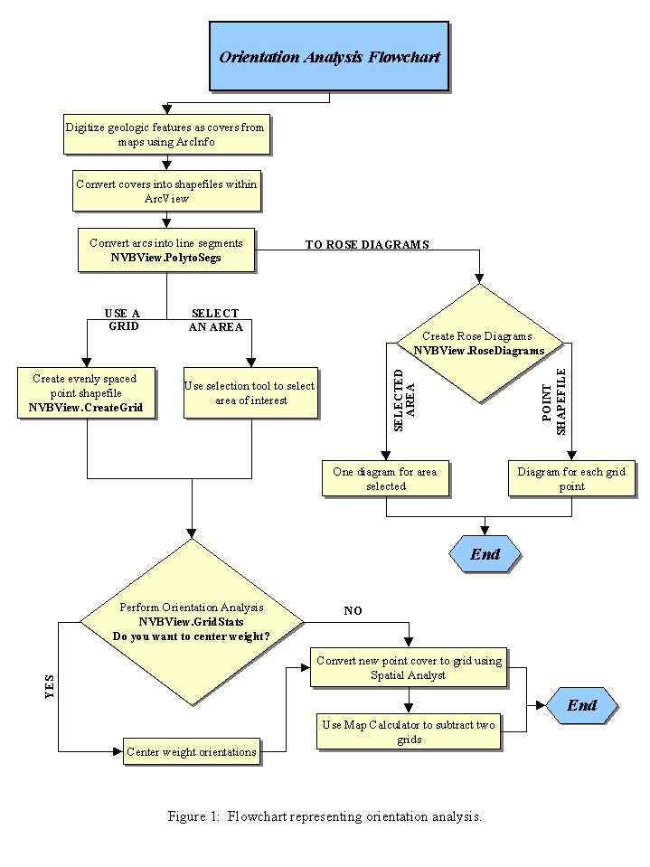
In order to analyze the orientation of geologic data represented as arcs, each arc needs to be broken into its individual line segments. This allows a more
rigorous description of an arc's shape because if an arc's orientation were calculated from its end points, there would be no difference between a line and an arc with
extreme changes in curvature. After the ARCINFO arc coverages are brought into ARCVIEW and converted into shapefiles, the script NVBView.PolytoSegs can
split each arc into its individual line segments. The end points of each line segment are then used to calculate the following variables (for orientation analyses): length,
line mid-point x- and y-values (to give a reference position for the line), azimuth (0 – 180o), 2 x azimuth (0 – 360o), sin(2 x azimuth), and cos(2 x azimuth). The
output for this script is a new line theme saved as
The next step is to define the spatial limits to be used in the selection of data and calculation of average orientations. The analyst can either manually select the
area over which to subdivide the data or define an evenly spaced point theme (or grid). For manual selection, the analyst uses the selection tool to choose the area
of interest. To define a grid, the script NVBView.CreateGrid creates a point shapefile by prompting the analyst to input the spacing in kilometers between each
point. From the bottom left corner (map origin), the spacing value, converted into meters, is added to x- and y-values until they exceed the extent of the view. The
script then builds a point theme (
The next step is to determine the orientation statistics for either the selected area or each analysis point. The third script, NVBView.GridStats, uses the selected area or prompts the analyst to input a selection radius from each analysis point that is used to select line segments with which to calculate the spatial statistics. For each analysis point, the script selects all line segments whose center points are within the selection radius distance from the analysis point. The analyst is then prompted to select either non-center weighted or center weighting (Eq. 1). Center weighting inversely weights the influence of each line segment by the distance between each line segment and the analysis point. For manually selected areas, the center of a selected area becomes the analysis point. The midpoint of each line segment is determined and the distance (L) from the grid point to the midpoint is calculated. Using the selection radius (R), the center-weighting factor is calculated as shown below:
Center Weighting Factor = CWF = (R – L) / R
Vector mean, resultant and dispersion values are calculated at each analysis point for the selected line segments using standard vector mean methods modified for lines (Davis, 1986). Lines cannot be averaged using straight vector mean calculations because northeast-trending lines can be represented as both 45o and 225o directions. The 2-theta method developed by Krumbein (1939) overcomes this problem by doing a vector mean of 2 times the angle and then dividing the final value by 2. For instance, 2 times 45o equals 90 o, as does 2 times 225 o (450 o -360 o =90 o). These calculations are performed in NVBView.PolytoSegs (Fig. 1). The equations to calculate the vector mean, resultant and dispersion in NVBView.GridStats are as follows:
Vector mean = [tan-1 (S sin(2*azimuth)*CWF*LLF / S cos(2*azimuth)*CWF*LLF)] / 2
Resultant = [(S change in x*CWF*LLF / n)2 + change in y*CWF*LLF / n)2]1/2
Dispersion = 1 – Resultant
where n represents the number of line segments, CWF is the center weighting factor (Eq. 1) and LLF (line length factor) is the line length, which weights the
calculation by the length of each selected line segment. To correct for the doubled azimuths in the 2-theta analysis and recover the true mean orientation, the vector
mean is divided in half. A new point theme (
The symbol plotted at each analysis point can be sized to correspond to increments of dispersion and colored to represent the vector mean using the legend
editor on the newly created point theme. A color scheme for 10o increments allows sufficient resolution for many analyses. Using ARCVIEW’s Spatial Analyst
extension, the point theme containing the statistical information (
Another way to represent the data is through rose diagrams. Rose diagrams give the analyst a graphical representation of the line orientations by a polar plot where the distance from the center of the plot is proportional to the sum of the line lengths in that orientation. Rose diagrams plotted with our script, NVBView.RoseDiagrams, plot a point for every 1o increment using two methods. To evaluate a specific area, the analyst can select line segments using the selection tool and create a rose diagram of all arc segments within this area. Alternatively, a user-defined radius around a point theme can be used. In either case, the analyst is prompted to define a smoothing increment that averages the length values for each degree by adding in values for adjoining degrees. For instance, the default smoothing increment of 10 o averages all the orientations five degrees before and after each degree.
ARCVIEW enhanced with the spatial analysis Avenue scripts (described above) was used to analyze the patterns of Laramide (70-40 Ma) deformation in the southern Rocky Mountains (New Mexico, Colorado, and Wyoming). Specifically, we wanted to test 1) if deformation patterns are consistent throughout the region and 2) if there was evidence for regionally consistent multi-phase deformation, which would be indicated by consistently multi-modal fold axis trends and multiple fault sets. ARCINFO was used to digitize faults and folds as arcs from United States Geological Survey 1x2 o degree quadrangle maps (1:250,000) and structural contour maps into a Universal Transverse Mercator, Zone 13, projection. These structures were digitized from maps of Wyoming, Colorado, New Mexico and parts of eastern Utah and Arizona.
Faults and folds were subdivided into four age groups to distinguish Laramide structures from those formed during Precambrian, Pennsylvanian, and Neogene orogenies (Table 1). The youngest rocks folded or offset by faulting were used to categorize the structures. Structures that involve post-Eocene rocks (<35 mya, type 1) indicate post-Laramide deformation and were excluded by this analysis. Type II, III, and IV structures all involve rocks that were present during the Laramide orogeny. Only type II structures were used in this analysis because type III and IV structures could have formed prior to the Laramide. We acknowledge that younger deformational events, such as those forming type I structures, may have contributed to some type II structures in areas where post-Eocene rocks have been removed by erosion.
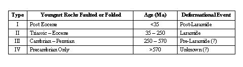
Table 1: Age categories of faults and folds.
A comparison of fault strikes (Fig. 2a) to fold trends (Fig. 2b) show that fault strikes are more variable. Fault strikes change from N-S in New Mexico to NW-SE in Colorado and WNW-ESE in Wyoming (Fig. 2a). At this state-by-state scale, multiple fault strike orientations can be seen, which was expected because synchronous thrust and strike-slip faults typically have different strikes even when they accomplish the same direction of shortening. The regional patterns of fold axes are less complicated, and do not show distinct changes in orientations, but multiple directions can be seen prominently in New Mexico and Wyoming and to some extent in Colorado (Fig. 2b).
To better detail changes in Laramide fold axis orientations, orientation analysis was performed on fold axes within Eocene to Triassic rocks (type II). The analysis was performed on 50 km analysis point spacing with a 100 km analysis radius and then converted into a grid that was used to display the vector mean orientations (Fig. 2c). In central New Mexico, a slight clockwise rotation from west to east is indicated in fold axis orientations from N-S to NNE-SSW. In Colorado, fold axes rotate more prominently clockwise west to east, from NW-SE to N-S. Fold axis orientations in Wyoming vary but are more consistently NW-SE. Data values are suspect in the easternmost portion of the grid due to the limited amount of data present.
The problem with using vector mean orientations to test whether multiple distinct fold axis orientations exist is that the vector mean calculations will average two or more modes of fold axes into an averaged orientation. To compensate for this problem, rose diagrams of fold axis orientations were created using 250 km for both their spacing and analysis radius (Fig. 2d). Overall, the rose diagrams are similar to the New Mexico, Colorado and Wyoming regional rose diagrams (Fig. 2b) and indicate unimodal distributions paralleling the vector mean orientations (Fig. 2c). With the exception of the most southeasterly rose diagram, which has a limited dataset, New Mexico fold axes show a dominant NNW-SSE trend with minor N-S and NE-SW modes also present. In Colorado, there is a clockwise rotation of the dominant trend from NW-SE in the west to NNW-SSE in the east. Southern Wyoming fold axis orientations show an overall NW-SE pattern and rose diagrams in northern Wyoming show a prominent NW-SE orientation with minor WNW-ESE and NNW-SSE orientations. The two easternmost diagrams in Wyoming are also suspect due to the limited amount of data represented.
The data indicate that type II, or Laramide, fault strike and fold axis orientations are broadly consistent at a regional scale but show important local variability. This suggests that caution should be used in extrapolating local results to the entire Rocky Mountain region. Multiple modes of fault strike and fold axis orientations support regional multi-phase, multi-directional hypotheses. Rose diagrams of fold axis orientations on a local scale vary throughout the area and also support multi-phase, multi-directional deformation hypotheses, although a NW or N trending mode is typically dominant with minor modes indicating other smaller events.
By adding Avenue scripts to ARCVIEW, orientation statistics can be performed on geologic map data. An evenly spaced point theme, or grid, can be used to calculate vector mean, resultant and dispersion values as well as smoothed rose diagrams. These values can be represented using color-coded grids created with the Spatial Analyst extension.
This quantitative approach reduces observer bias and can be used to test geological hypotheses by calculating the angular differences of geologic map data such as faults and folds. When applied to Laramide deformation in the Rocky Mountains, these tools indicate gradual, systematic changes in Laramide fault and fold orientations. Initial results support moderate changes in Laramide shortening directions in the Rocky Mountains of New Mexico, Colorado and Wyoming. This example shows how the addition of spatial analysis tools to GIS representations of geological maps can transform them from static spatial data to dynamic tools that quantify geologic history.
We thank David Theobald at Colorado State University for Avenue programming help. We would also like to thank the Rocky Mountain Map Company in Wyoming for supplying the structural contour maps used for this project. Funding was provided as a supplement to the N.S.F. Continental Dynamics – Rocky Mountain Project Grant EAR-9614787 awarded to Karl Karlstrom of the University of New Mexico and N.S.F. grant EAR-9814698.
Bird, P., 1998, Kinematic history of the Laramide orogeny in latitudes 35o - 49oN, western United States: Tectonics, v. 17, p. 780-801.
Brown, W.G., 1988, Deformation style of Laramide uplifts in the Wyoming foreland, in Schmidt, C.J., and Perry, W.J., Jr., (eds.), Interaction of the Rocky Mountain foreland and the Cordilleran thrust belt: Geological Society of America Memoir 171, p. 53-64.
Cather, S.M., 1999, Implications of Jurassic and Cretaceous piercing lines for Laramide oblique slip faulting in New Mexico and the rotation of the Colorado Plateau: G.S.A. Bulletin, v. 111, p. 849-868.
Chapin, C.E., and Cather, S.M., 1981, Eocene tectonism and sedimentation in the Colorado Plateau-Rocky Mountain area: Arizona Geological Digest, v. 14, p. 175-198.
Davis, J.C., 1986, Statistics and data analysis in geology, 2nd ed., John Wiley and Sons, Inc., New York, p. 320-321.
Erslev, E., 1993, Thrusts, backthrusts and detachment of Laramide foreland arches, in Schmidt, C.J., Chase, R., and Erslev, E.A., eds., Laramide basement deformation in the Rocky Mountain foreland of the western United States: GSA Special Paper 280, p. 125-146.
Erslev, E.A., and Wiechelman, D., 1997, Fault and fold orientations in the central Rocky Mountains of Colorado and Utah: in Hoak, T.E., Klawitter, A.L., and Bloomquist, P.K. (eds.) Fractured Reservoirs: Characterization and Modeling: Rocky Mountain Association of Geologists 1997 Guidebook, p. 131-136.
Gries, R.R., 1983, North-south compression of the Rocky Mountain foreland structures, in Lowell, J.D., and Gries, R.R., eds., Rocky Mountain foreland basins and uplifts: Rocky Mountain Association of Geologist, Denver, Colorado, p. 9-32.
Krumbein, W.C., 1939, Preferred orientation of pebbles in sedimentary deposits: Journal of Geology, v. 47, p. 673-706.