Psomas is a mid-sized Survey and Engineering firm providing GIS and Environmental services to a diverse spectrum of private and municipal clients. Obtaining low cost, spatially accurate digital base map data is often a critical first step in the development of GIS services and applications. Although a variety of low cost data sources exist, USGS digital sources have proven to be unparalleled in their level of accuracy, detail, and accessibility. This paper introduces the vector and raster base map data available from the USGS, and discusses their potential uses and applications.

INTRODUCTION

Throughout the history of the United States, maps have played a pivotal role in the development of our nation. There is virtually no aspect of commerce, environment, or politics that is not in some integral way related to its physical location, or does not derive its essential nature from the geospatial context of its surroundings. The USGS 7.5 minute quad sheet, usually referred to simply as a USGS "quad" or "topo map", has become the workhorse of most common mapping applications. On any given day thousands of quads lie spread out on the desks of planners, engineers, biologists, economists, historians, politicians, recreational enthusiasts, and of course geographers, playing an integral role in whatever task is at hand. They have become so common and easily accessible that we run the risk of taking them for granted, and lose sight of the technical, logistic and monetary effort that was needed to produce them in the first place.

Today, the base mapping of the United States and its territories at 1:24000 scale is completed—a total of over 53,000 individual qaud sheets delineating transportation (roads, railroads, utility features, and pipelines); hydrography ( lakes, rivers, reservoirs, dams, wells and springs); hypsography (elevation contours and spot heights); boundaries (of counties, cities, national parks, national forests, reservations and other municipalities); public lands (the public land survey system depicting section, range and township locations); vegetation (forests, shrubland, wetlands, and agriculture); man-made features (buildings, airports, stadiums etc.); non-man-made features (sand dunes, glaciers); survey control (horizontal and vertical control of the National Geodetic Network); geographic names (of all of the features above, including cities, rivers, mountains, canyons, etc.) and coordinate grids, in Latitude/Longitude, Stateplane and UTM projections. The private-sector cost of creating today a single 24K quad depicting the same information, and produced to meet National Map Accuracy Standards, has been estimated at approximately half a million dollars. Yet anyone can buy such a map, in full-color 24 x 36 inch format, for four dollars and fifty cents. It would be difficult to find any product in the public or private sector of comparable cost and benefit. The foresight, productivity and public service of this agency is probably without peer in the government sector. We owe to them an incalculable debt.

Several decades ago the USGS embarked on the journey of developing a model to convert its hard copy maps into digital format. Based on the simple concept of cartesian coordinate systems, and extended to include concepts of topology, the "Digital Line Graph" was born. These vector based mapping data represented the first mass produced GIS data for public use in the world. As both funding and need grew, so did the extent of the digital data program. The program was extended to include production of digital elevation models (DEM's), scanned USGS topo maps (DRG's), and digital orthophotography (DOQQ's). Taken as a whole, these core datasets of the so-called "National Framework" probably represents the lowest cost, highest quality, and most underutilized digital GIS basemapping data currently available.

There is a reason why USGS digital data is not used as much as it could be: it is notoriously difficult and time consuming to process. In fact in the absence of platform specific programs (e.g., aml's) developed specifically for the purpose of processing the data, the routine use of the data for GIS basemapping applications is for most intents and purposes impractical. This is an impediment in its own right but has led to another, perhaps more serious problem in terms of public awareness--the average GIS user has probably only a passing familiarity with the benefits of using the full suite of data available from the USGS precisely because it is so difficult to process. And while any of the data sets taken individually can be useful, their true power is realized when they are routinely used as a total basemapping "package".

This paper is not intended to be a data processing handbook. The intent is to introduce, or perhaps re-introduce, the various commonly available USGS datasets. The sections that follow will outline some of their advantages, in the hope that readers will become interested in their use. The following two tables describe the datasets discussed in this paper, where to get them, and how much they cost.

Available Products

Where to Get Them

Digital Line Graphs (commonly known as "DLG’s) are a digital vector representation of the features typically seen on a standard USGS topographic map. Unlike a scanned quad sheet, which is simply a graphic image, these vector data sets can be converted into actual ArcInfo coverages. Each layer can be edited and cartographically manipulated, for example to update the alignment of a road or to change its display characteristics. DLG's are available three different scales: 1:24,000 (24K), 1:100,000 (100K), and 1:2,000,000 (2M). This section focuses on the 100K DLG product because of its wide availability. 100K DLG’s come in 5 separate data sets representing a total of 10 different data layers as listed in the table below.

Coverage layers for USGS DLG 100K data.

The principle advantage of DLG’s is that they are the only seamless vector basemap data in the United States produced to meet National Map Accuracy Standards. This means that on a regional scale, adjoining map sheets will meet at their edges, and features will have uniform accuracy at scale. This is an important consideration in regional mapping applications, where uniform basemap data is needed to cover tens or hundreds of miles. DLG data also tends to have a higher resolution than comparable data sets of national scope. For example, coastlines and lake shorelines show a great deal of detail when compared to other more generalized data sets. In fact the term "100K" scale is somewhat misleading. 100K DLG data sets were originally compiled from 1:24,000 (24K) topo source sheets, and although certain feature classes were weeded out—for example vegetation and man-made features—others were retatined at virtually full resolution. For example in the DLG Transportation layer, road detail is retained to the level of residential streets.

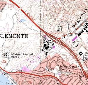
"100K" DLG residential roads layer (in magenta) overlayed on 24K DRG

DLG data can also be described as "feature rich". There is no other data set of national scope produced to meet NMAS that contains the unique combination of basic base mappping layers as listed in the table above. And although most applications will probably never need to know the locations of duck ponds, railroad sidings, or meander corners, there many types of data contained in DLGs which can be found nowhere else. The sections that follow include an outline of the major feature types included in each of the 100K DLG data sets. The most commonly sited drawback to DLGs is their vintage. Most DLG 100K is more than a decade old, and a lack of funding has held back systematic updating and revision of the data. This is less of a problem in rural areas or in urban areas which have been "built out", where major features may change little. But it is an issue in developing areas where many new features-- particularly transportation features and municipal boundaries-- may not be current. Even in such situations it's usually better to start with an existing digital map that can revised than to start with nothing at all, and features can be revised by referring to other reference information such as current aerial photography. The USGS DOQQs are particularly useful for this purpose since they are both digital and fully orthorectified. DLG’s are also notoriously poor in some types of attributing. For example, attributes will exist to distinguish a major road from a trail, or a river from a shoreline, but the proper names of features are rarely attributed. This can be a major issue for themes such as roads or hydrography, where feature names can be vital to the purpose of the map; the manual addition of correct attributing from alternative reference maps can be extremely costly and time consuming. Not all DLG data layers are subject to these limitations. For example, the Public Land Survey System layer is fully attributed with section, range and township information. The Miscellaneous Transportation layer, although not fully attributed, may be less of an issue since features such as power lines, pipelines and railroads are relatively few and relatively easy to attribute manually.

The sections below list the feature attributes present in each data layer along with some sample graphics intented to give the reader some feeling for the degree of feature richness present in DLG datasets.

Roads and Trails

Contours

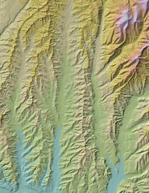
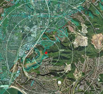
Digital Elevation Models (commonly referred to as DEMs) are a raster-based grid of numeric elevation values. They are used in a GIS to produce three-dimensional terrain models. Because they are based on a raster data model, some products produced from DEMs can appear similar to simple graphic images. For example, DEMs are commonly used to produce striking shaded-relief images, which in addition to their visual appeal, are extremely useful for visualizing local and regional terrain features. But DEMs are more than simple graphic images. They are fully georeferenced coverages and can be used to produce numerous spatial and analytical products. For example, DEMs can be used to produce maps of slope and aspect, and can be used to generate vector elevation contour lines. They are also the foundational data set used in many terrain-based GIS modeling applications such as watershed modeling, visibility analysis, flood susceptibility, landslide potential, and wildlife corridor determinations.

DEMs are distributed in two common scales. 24K DEMs (also known as 7.5 minute or 1:24,000 DEMs) cover the extent of a standard 7.5 minute, 1:24,000 USGS quad sheet. The nominal grid cell sampling resolution can be either 10 or 30 meters. 250K DEMs (also known as 3’ – "three second" or "three arc second" DEMs) cover the extent of a standard 1^o, 1:250,000 USGS quad sheet. The nominal grid cell sampling resolution is three arc seconds, a distance of about 90 meters. The use of one product versus the other depends on the application. 24K DEMs cover a smaller area of the earth’s surface, and have a correspondingly higher degree of accuracy and resolution than the 250K DEMs. As such, they are generally the preferred product for modeling and analytical applications on a local or semi-regional scale. If the study area is larger than a single quad sheet, adjoining DEMs are usually mosaiced together into a single, larger DEM. The larger the study area, the more DEMs that must be mosaiced, and the larger the output DEM becomes. For example, a single 24K DEM (floating point) has a size of roughly 10 Megs; mosaicing 10 DEMs together will produce an output DEM of about 100 Megs. At some point, the output DEM becomes too large to be practical, and the use of the 250K DEM product may be preferred. The 250K DEM has lower accuracy and resolution than the 24K DEM, but it covers a much larger area without incurring the larger file size. They are useful for regional modeling applications, and they are excellent cartographic tools for producing three -dimensional vicinity maps to show local study areas within their broader, regional context. They can also be useful as an overlay tool for producing perspective photographic drapes.

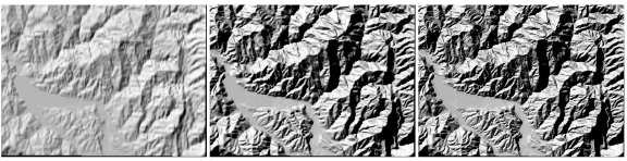
24K DEMs are produced in 3 different levels of accuracy and resolution: 30 meter, level 1; 30 meter, level 2; and 10 meter, level 2. Level 2 data is collected with different methods than level 1 and is generally both more accurate and of higher visual resolution on-screen than level 1. 30 meter coverage is available for the coterminous US. 10 meter 24K DEM coverage is relatively rare, but if you can find it where you need it is of exceptional quality. The graphic below shows a comparasion between 30 meter, level 1; 30 meter, level 2; and 10 meter, level 2 data for the same quad.

There are several caveats worth mentioning in the processing of DEM data. There is no standard vertical unit in the production of DEMs. Native horizontal units are meters, but vertical units can be either meters or feet, depending on the extent of the local terrain relief. As a consequence, a neighborhood of adjacent DEM's are frequently of mixed vertical units and must be converted to a standard vertical unit during processing. The USGS also uses two different integer values to represent areas of "no data". Null data areas are coded with the value -32,766 while void data areas are coded with the value -32,767. If these values are not replaced with valid ArcInfo "no data" values they will be interpreted as elevations, and corrupt the DEM during conversion. Lastly is the issue of vertical datum. Just as vector coverages must always specify a horizontal datum as an integral part of the projection parameters, the vertical datum is equally critical when dealing with DEM elevation data. Unfortunately, ArcInfo does not currently support reporting of the vertical datum as part of the conversion process. The standard vertical datum for 24K DEMs is the North American Vertical Datum of 1929 (NAVD29). Native elevations can be converted to the more current North American Vertical Datum of 1988 using a quad specific conversion factor obtained from the USGS. With the advent and proliferation of GPS data, which commonly uses NAVD88 as its datum, conformance to a common datum is critical.

USGS Digital Raster Graphics (commonly known as DRGs) are scanned, geo-referenced images of standard 7.5 minute USGS quad sheets. They are not vector coverages—they are simply images—but they differ from a simple graphic picture in that they are geo-referenced. When correctly projected, DRGs will "overlay" with all other GIS data layers in correct geographic space. The images are in full color and high resolution. In fact, plots of DRGs from an HP 2500 plotter are virtually indistinguishable from the original paper product.

DRGs have a variety of uses. The most obvious is that, in digital form, color copies can plotted and distributed at will. Derivative products, such as project specific features overlaid onto the DRG and replotted, are easily produced. This is extremely useful for field personell such as surveyors, biologist, geologists, and so on who routinely use topo maps in the course of their work. Since most people are already familiar with the "look" of a standard USGS 7.5 minute quad sheet, DRGs are also useful as background images upon which specific GIS data layers can be overlaid. Using DRGs in this way is often a cost-effective solution to creating quick exhibits, since the overhead of creating all of the background detail—roads, streams, major buildings, etc.—is avoided.

Native DRGs are "collared"; the product looks identical to a standard USGS topo map and includes the white paper margin surrounding all USGS quad sheets. The collar contains a variety of standard USGS information such as the title block, the scale bar and north arrow, the names of the four surrounding quad sheets, the coordinate system grids for Latitude and Longitude, State Plane, and UTM projections, and so on. This information is often vital to a user, and its inclusion makes it possible to reproduce a USGS quad sheet in full fidelity.

Metadata contained in the margin or "collar" of a native DRG.

For the purpose of screen display or GIS overlay mapping however, the collar often gets in the way. For example, if a user wants to display two adjacent DRGs on-screen at the same time, the white collar of one DRG will overlap, and effectively cover up, the mapping data on the adjoining DRG. To solve this problem, the collar can be clipped to form a "collarless" DRG. This makes it possible to load multiple DRG simultaneously with no loss of information. It is also an effective solution for producing overlay exhibits across multiple quad sheets—adjoining quad sheets will appear "seamed" together into one consistent map.

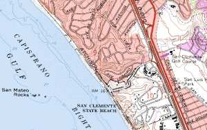
Collarless DRGs displayed as a single mosaic.

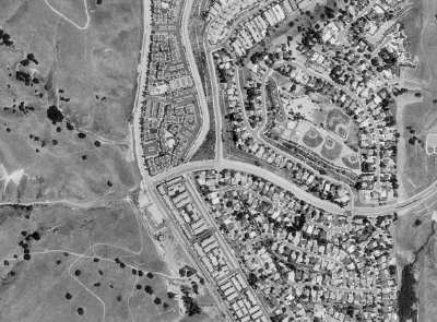
USGS Digital Orthophoto Quarter Quads (typically called "DOQQs") are georeferenced, fully orthorectified, digital aerial photography. Because the effects of rotation, tilt and terrain relief have been removed they can be used directly for feature digitization and GIS data layer updating. They are extremely useful as an overlay for verifying, revising, and supplementing the information content of DLGs, DRGs, and DEMs. They are also an invaluable tool in the field as an aid to regional and urban planning efforts and environmental mapping projects. The imagery has a native resolution of 1m and will support plots to scales of 1:3,000 (1"=250’). Because file sizes are large (typically 50 megs for black and white and 150 megs for CIR), they are distributed as quarter sections (NW,NE,SW,SE) of a 7.5 minute quad sheet.

Unlike DRGs, DOQQs have no collar and are intentionally produced with a good degree of overlap between adjacent images. Native DOQQs are generally not color balanced, so the "seam" between images may visible as a discrepency in tone and contratst even though the geometry is solid. Image processing software can be used to feather and color balance adjacent images if necessarry.

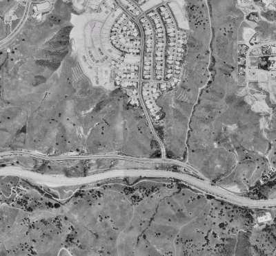
Adjacent DOQQs showing slight differences in tone and contrast.

DOQQs are generally flown on a five year cycle. More current orthophotography can be obtained on the open market but would typically cost several thousands of dollars for comparable "custom flown" orthophotography. The fact that DOQQs can be purchased for a base charge of $30.00 at $7.50 each makes them a remarkable resource.

CONCLUSION

In summary, the core National Framework datasets—DLGs,DEMs,DOQQs and DRGs—constitute a powerful and versatile suite of GIS basemapping and analytical tools that would not otherwise be available, except at enormous cost. Their underutilization by the general GIS community is undoubtedly related to the difficulty, time and effort associated with processing the data into a useful product, but more people might make that effort if it were clear what the benefits are. In our experience, there is rarely a project that is not benefited by the use of these datasets, frequently for the performance of value added services which budgetary constraints would not otherwise have allowed. With each dataset georeferenced and produced to consistent National Map Accuracy Standards, they represent the most consistently accurate, lowest cost and readily available data of its kind.

Duane Haselfeld

PSOMAS

3187 Red Hill Ave., Ste. 250

Costa Mesa, CA 92626

714-751-7373