
The workshops serve several purposes, including helping to develop a "Planning Toolkit," consisting of software modules and tools which help support land use analysis, growth allocation, visualization, and impact assessment. Through an electronic interface, the toolkit will enable citizens to better understand, visualize, and predict future consequences of alternative land use plans. Partners in this project include Dane County and the University of Wisconsin-Madison, along with both the City of Verona and Town of Verona, Wisconsin.
Since September 1998, we have taught 15 classes to approximately 231 students on the use of GIS for land use planning. The majority of students have been from Dane County or other agencies/departments statewide. However, several classes have been customized for training at other locations through our mobile training lab. These include classes held in Portage County, WI, Door County, WI, Pennsylvania (focused on farmland preservation), and 2 separate courses for the Wisconsin Land Information Association Annual Conference. We have received very positive feedback from those who have taken the courses on material presented and its use in land use planning.
The course is instructor and staff intensive, involving at least 9 individuals in its teaching and development. There are typically 3-4 instructors, and between 10 and 25 participants. The Planning Analyst consists of 5 "Modules"
Early inventories of the landscape revealed regional patterns of slopes, wetlands and surface waters. Professor Lewis reasoned that, if protected, these land patterns could act as "form determinants" to guide future growth. By plotting our water, wetlands, and steep topography (12.5 percent slope or greater) within an integrated system, we can classify these patterns as "environmental corridors." Professor Lewis suggested that environmental corridors could then be used to establish priority zones for future studies as a means to guide growth.
By working with local citizens, he developed 220 icons that depict specific natural and cultural features ranging from quality fish habitat to historic buildings. He found that 90 percent of these features were found within the corridors containing the water, wetlands, and steep slopes. Lewis called these particular areas "nodes of diversity." His message was this: instead of fighting for one particular resource, we should protect and enhance the corridors that contain a variety of features and values we want to protect.
The basic model calls for the combination of surface waters, steep slopes, and wetlands. Additional factors can include forests, floodplains, prairies, parks, or regionally determined factors like beaches, dunes, geological formations, etc. In Dane County, the Water, Wetlands, and steeps slopes look like this:
(Figure 1. Dane County)
In Model Builder, the original model, which simply finds the union of the areas in the 3 layers, is elementary. A more interesting model includes existing protected areas, uses distance from all the layers as well, and takes into account threats to environmental corridors such as proximity to urban factors.

(Figure 2. Environmental Corridors Core Model)
A model for Environmental Corridors has been developed, but not incorporated into the Landuse Planning class yet. It is expected to be introduced for the next class, in August of 2000.
Despite the importance of farming to our economy and quality of life, Wisconsin is losing farmland at an alarming rate: approximately 100,000 acres of farmland each year. Dane County alone is losing more than 3,000 acres annually (Design Dane! 1998). Preserving farmland, and farming, poses a huge challenge to Dane County, the state and the nation. Volatile markets and development pressures have persuaded many to sell their land and forsake farming as a livelihood.
This model provides more variables, and more decisions based on personal preferences to determining the outcomes. Participants were introduced to some of the concepts, and given a 3-step process to establish Farm Priority Zones (FPZ): 1) Construct a base layer; 2) Derive potential FPZs; and 3) Evaluate and select final FPZs.
1) Constructing a Base Layer for Analysis. The model begins with identifying actual farms. Data are selected and organized to fit a local definition of "farmland." This base layer is the foundation for running the preservation model. Defining farmland is not always simple and straightforward. The U.S. Department of Agriculture developed the Land Evaluation and Site Assessment (LESA) model to help communities sort through the complex issues surrounding farmland preservation. LESA consists of two portions: Land Evaluation (LE) describes the physical properties of farmland. This includes soil productivity, land capability factors such as erosion, and important farmland designations. Site Assessment (SA) includes cultural factors such as economic productivity, development pressures, as well as public values supporting preservation. The LESA model allocates priority to factors by assigning "weights" and scores. For example, high-quality soils are assigned a higher-value score than low-quality (less productive) soils. These designations, if available, can help determine which lands to assign to the agricultural base layer. Lands being assessed as agricultural for tax purposes, or those in Agricultural zoning give another or refine the set. Potentially, all lands in agriculture at present could be included in the Base Layer, or only those that meet some criteria: Minimum size, Exclusive ag zoning, LE score over a threshold, etc.
2) Deriving Farmland Priority Zones. Other factors influencing agriculture are added, and assigned weights in the model. These might include Biophysical elements, such as geology, land cover, flood plains, groundwater, climate, and pests; or Demographic and Locational Patterns, like population and housing densities; or agricultural demographics such as number of farms per zip code. These data can help locate where the agricultural sector is prominent or where urban conditions prevail.
In urbanizing areas, a farmland preservation plan should consider urban determinants such as development patterns carefully. Close proximity to rural residences, urban service areas, and municipal boundaries may increase development pressures on farmland. This is generally due to lower development costs and close contact to urban amenities such as water and sewer. In the urbanizing rural landscape, pressures may also come from people seeking aesthetic amenities like open space and larger tracts of less-expensive land.
Preservation tactics in agriculturally prominent areas should focus on patterns important to agriculture. Distance to markets and agricultural services may be important. And in both farm areas and newly urbanizing areas, farmland that comprises a large contiguous area may be the pattern most worth mapping and preserving. Why? Because large areas are generally more productive, bear fewer urban pressures such as traffic, and offer a broader rural aesthetic presence.
3) Compare the FPZ with other data and field verification.
Participants in our Landuse Planning classes were given a simplified model of one township to run using the Model Builder. (see figures 1 and 2)
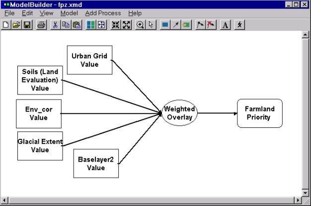
(Figure 3 FPZ Model)
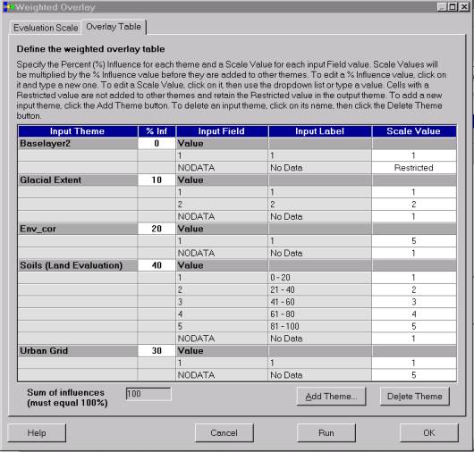
(Figure 4 FPZ Model Weights)
Participants were presented with descriptions and hands-on exercises involving theme-on-theme selection, attribute query, and shapefile creation in the original class schedule. With Model Builder, we had the opportunity to present them instead with a model where they could set their own ranking for the suitability of features and layers to agriculture, in a single interface. Feedback from the participants suggests that this method is easier to understand than the previous, and that it is also much easier to make changes to if the results do not match expectation, or if different values for the parameters are desired.
A more complex model still being tested will include creating a base layer, and some of the model layers, using more sophisticated GIS functions.
This analysis began as a way of identifying how much land was available for development. Since many of the factors listed above can occur on the same piece of land, it was necessary to prioritize them, and create output that had a single use for each unit of the landscape. This was much easier to do in the ArcView Spatial Analyst than in a vector environment, and so it was. Each layer was converted to a grid with a unique value for presence, and nodata for absence of each factor. These were then merged in the following order, thus establishing priority:
Residential, Mercantile or Industrial, then
Since each input grid had a unique value, the result had a unique value for each grid cell representing its use. These are summed up and multiplied by the cell size to give total areas in each category, which is what we were originally searching for.
This method does not account for multiple factors. One way to do so would be to have a value of 1 for each factor except the "background" layer of Ag/rural, which would get a 0, and then sum the grids. The value in each grid cell then becomes the number of factors. All those with a value of 1 or greater have at least one growth management factor, and those with multiple factors will have correspondingly larger values. This calculation does not allow one to know which factor is at a location, however.
A further alternative is to assign a unique number to each factor, where the number is a power of 2 - 1, 2, 4, 8, 16, 32, etc. Then when the grids are summed, the total gives a unique value, depending on which layers contributed. This is easies to illustrate if you view the numbers in their binary representation. Say you have a 1, a 4, and a 16, the sum is 21 seen as base 10, but in base 2 notation, they are 1, 100, and 10000, giving 10101. Thus, the placement of the 1's indicates the contributing layer.
These three methods each have a value, and each tells something different about the area being studied. None of them is the weighted overlay model that is used in the Model Builder, either. That model is intended for assigning a suitability value for each of the input criteria. So to use the functions of the Model Builder, a slightly different model was developed.
For this model, we used a smaller area, selected for the Shaping Dane's Future project, which included the Township of Verona, plus a 1 ring 1 section ( ~ 1 mile) wide around the town.
The input data sets included the ones above, as well as the following:
These data sets can be viewed at the Shaping Dane web site, at the URL: http://www.lic.wisc.edu/shapingdane/, or directly at:
http://www.lic.wisc.edu/shapingdane/resources/atlas/data/frames-data.htm
To make the model more complex (and interesting), we did not use simple presence/absence data for some of the themes. For instance, rather than using a slope map that was simply slopes greater than 12%, we took the DEM and reclassified slopes into 5 classes, at 0-5, 5-8, 8-12, 12-20, and over 20%. With these categories (or others the participants could redefine), ratings for suitablility for development could be established. Similarly, the layers for environmental Corridors, Forest, Iceage Trail Corridor, and a buffer around parks are summed to give a high value where multiple features occur. Here is that model:

Acknowledgments
The author would like to acknowledge Doug Miskoviak for help testing and evaluating the Model Builder; the Director, Associate Director and the rest of the LICGF for providing both a facility and an environment conducive to learning and developing ideas, and fertile ground for projects like this one; and Dane County, for providing most of the data usedin these classes.
References:
Design Dane! Creating a Diverse Environment through Sensible, Intelligent Growth Now. 1998. Dane County Planning Department. Madison, Wisconsin.