LIDAR (LIght Detection And Ranging) data sets for forest evaluation are characterized by systematic data collection using a high-performance, photogrammetric Laser Pulsing System; the capability to record Multiple Returns; and, the capacity to collect, manage, and store remarkably large data files. Quality assurance of the raw data based upon accepted accuracy measurement techniques is critical before post-processing of the data can begin.
Substantial efforts in post-processing LIDAR for Northwest Forestry Applications have demonstrated the value of the technology for delineation of the bare ground (DEM – Digital Elevation Model) and the canopy layer (SEM- Surface Elevation Model). This paper presents current results of assessments of accurate, multi-return LIDAR data, and quantifying the results to determine forest conditions. The results will be presented with effectual graphics in an ArcView environment to communicate the usefulness of LIDAR for forest assessment and data applications.The development of airborne laser scanning goes back to the 1970s with early NASA systems. Although cumbersome, expensive, and limited to specific applications (such as simply measuring the accurate height of an aircraft over the earth’s surface), these early systems demonstrated the value of the technology. By emitting a laser pulse and precisely measuring the return time to the source, the “range” can be calculated using the value for the speed of light (similar to a total station surveying instrument).
The advent of GPS measuring systems in the late-80s provided the necessary positioning accuracy required for high performance LIDAR. It wasn’t long until rapid pulsing laser scanners were developed linked to the GPS system. The systems became complete with ultra-accurate clocks (for timing the return) and Inertial Measurement Units (IMU) for capturing the orientation parameters (tip, tilt, and roll angles) of the scanner.
A modern LIDAR system has a rapid pulsing laser scanner (with continuous wave lasers which obtain range values by phase measurements), precise kinematic GPS positioning, orientation parameters from the IMU, a timing device (clock) capable of recording travel times to within 0.2 of a nanosecond, a suite of robust portable computers, and substantial data storage (100 GB).
From the earliest applications of airborne laser scanning, the mapping community was aware that vertical accuracies of a 15 cm RMSE were possible, with horizontal accuracies at about two times the footprint size. Maximizing this technology greatly reduces the time and fieldwork effort required by traditional methods.
Modern LIDAR systems are the result of rapid advances in technology during the last several years.
The Scanner:High-performance scanners are capable of emitting up to 15,000 pulses per second with a variable-scanning angle of 1( to 75(. With continuous wave laser pulses, multiple return values for each pulse may be recorded – up to 5 return values per pulse. Operating in the near infrared (1064 nm), pulse values may be recorded after diffusion and reflection on the ground. GPS and IMU technology is integrated into the scanner, as well as, a robust timing mechanism (clock). In addition to recording returned pulse range values, some scanners also provide signal intensity, amplitude, and pulse angle.
GPS and IMU and Timing ClockPrecise kinematic positioning by differential GPS and orientation parameters by the IMU of the scanner is critical to the performance of the LIDAR system. The GPS provides the coordinates of the laser source (the scanner) and the IMU provides the direction of the pulse. With the ranging data accurately measured and time-tagged by the Clock, the position of the “return point” can be calculated.
SoftwareThe four primary components of a LIDAR system (Scanner, GPS, IMU and Clock) each operate within an independent plane-of-reference. As a result, the assembly of components requires sophisticated software for accurate intercommunication. The delivery of each pulse carries a time tag, position value, and orientation parameters. Multiple returns from each pulse require cataloging and a nearly perfect storage protocol. In some cases the hardware manufacturers provide a complete system with software; the highest performance systems usually require custom software for component integration.
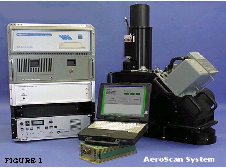
Computer SupportEach primary component requires dedicated computer support – scanner, GPS, and the IMU. In addition, another computer supports the aircraft navigation, and another acts as a server with significant data storage. Figure 1 is a composite illustration of the AeroScan LIDAR System showing the Scanner, IMU, and supporting hardware.
Once the system is assembled, a “bore sight” is required for calibration. By collecting LIDAR data of a pre-measured target(s), the performance (internal referencing) of the system is modeled, so that the configuration of the components (as installed) is known. These values are used in post-processing to calculate the accurate location for LIDAR return values to an external referencing system. Each time the system is removed, a new bore sight is required.
LIDAR data collection begins with a well-defined flight plan meeting the project’s requirements. The average post-spacing of the points must be at a density to support the level required for a Digital Terrain Model (DTM) or Surface Terrain Model (STM). The density of post-spacing may be modified by changing the flight altitude or the scan angle. Urban areas with tall buildings and steep terrain require special consideration to avoid holes in the data.
For the kinematic GPS, a base station of known location with a multi-channel GPS must be initialized with the on-board LIDAR GPS receiver. This initialization lock must remain in place during the entire flight mission. For this reason, very shallow turns are made between flight lines during the data acquisition.
LIDAR data may be acquired quite rapidly: a system emitting 15,000 pulses per second with the capability to record 5 returns per pulse could potentially capture 75,000 values per second. In reality, the number of returns from such a system collecting data for a NW forest is closer to 35,000 values per second. At 900,000 pulses per minute, a typical 3-hour mission results in about 120 million pulses.
Since LIDAR is an active illumination system, data can be captured in all ‘clear’ conditions – day or night. This factor is very useful in taking advantage of good weather conditions and the opportunity to capture data at night in busy air space areas around airports. As mentioned, most terrain mapping LIDAR systems use a near infrared laser, so pulses hitting standing water are absorbed.
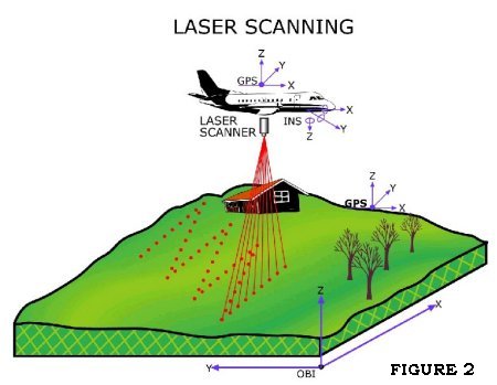
Upon landing after a mission, the system is de-initialized, and quality assurance of the data begins. Since all of the data collected is geo-referenced, it can be viewed in-situ using ArcView to verify coverages of the subject site. Also, to validate the accuracy of the collection, known survey data and a check of the bore site should be completed in-situ. Without proper quality assurance at this phase, the absolute accuracy of the data collected is suspect to error. Figure 2 summarizes the operational characteristics of LIDAR data collection.
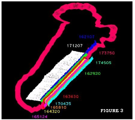
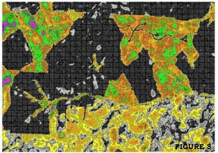
LIDAR data pre-processing is composed of two efforts. First, the data must be filtered for noise, differentially corrected (as with any high accuracy GPS survey), and assembled into flight lines by ‘return layer’. This processing computes the laser point coordinates from the independent data parameters: scanner position, orientation parameters, scanner angular deflection, and the laser pulse time of flight or slant range. LIDAR data sets are remarkably large point files. Most LIDAR providers assemble the returns as a basic ASCII file of x, y, and z values which have been transformed into a local reference coordinate system. A typical flight line six miles long with a 40( scan width produces an ASCII file of about 5 MB for 1st return values only. Robust data processing hardware is a fundamental requirement. Figure 3 illustrates an immediate data collection validation procedure which converts a portion of the LIDAR points (thinned) to a raster file for display in ArcView. Note that the data recorder was not disabled while the aircraft turned (pink flight line) showing the complete flight path for this single pass.
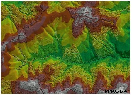
Second, the LIDAR data must undergo further analysis to derive the final products – DEM, SEM, or intermediate return information. These surfaces are derived using skilled technical staff and ArcView/3D Analyst. Current aerial photography, imagery, and existing maps are required to deriving these products with a high confidence level. Figure 4 is a Triangulated Irregular Network (TIN) of ‘first-return’ LIDAR for a forested site.
If current imagery is not available, collecting geo-referenced 4k x 4k digital CCD imagery (integrated to the same IMU and ABGPS as the scanner) with a calibrated camera/lens is effective. This imagery may be quickly ortho-rectified using the captured orientation parameters (without aerotriangulation) and the LIDAR DEM.
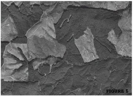
Post-processing progresses more effectively and with higher confidence. Mapping forests exhibiting a diversity of management treatment options are processed quite effectively through the combination of digital imagery and LIDAR. Figure 5 is a digital orthophoto of the forestry site which was generated from an image flown before the LIDAR collection. The orientation parameters from this image and the LIDAR DEM were used to rectify the image.
Firms providing LIDAR services typically have developed a suite of in-house algorithms for deriving the canopy (or SEM) and a bare earth DEM. These software modules analyze the multi-surfaces mapped by the multiple return LIDAR data sets. The processing for bare earth begins with the LIDAR points with the highest likelihood of being on or near the earth’s surface. The LIDAR Analyst proceeds by moving from the “known to the unknown”, making reference to the imagery, and removing aboveground points selectively.
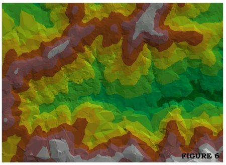
Figure 6 is a TIN of the bare earth DEM for the forestry site. For this four square mile area, much of which is covered with mature forest, the level of LIDAR point density supported 20’ contours throughout. Most of the area contained 10’ supplemental contours.
As a final check, representative sites within the project area should be verified photogrammetrically on a stereo plotter. LIDAR points are easily visible on the 3D stereo model for analysis, and from this check an accuracy statement for the data set can be developed for the final Report of Survey.
Data delivery is usually in a format ready-for-use for GIS applications in the correct coordinate system. Existing accuracy standards should be utilized to the greatest extent possible: the ASPRS Large Scale Mapping Standard and the National Spatial Data Accuracy Standard. For example, if the density of ‘ground points’ does not support the accuracy required, these areas should be annotated and noted for low confidence.
To accompany the deliverables a Record Of Survey should outline the procedures for data collection and post-processing, the intended post-spacing, flight parameters, kinematic GPS reports, and referencing of the base station.
LIDAR technology has provided mapping professionals with a very useful tool for quickly acquiring a wealth of data for the surfaces(s) of the earth. Mapping in forests for the first surface (canopy) and deriving a bare earth DEM from ground LIDAR points is of great value to the forest managers developing vegetation cover maps and surface models (slope, aspect, hydrology models, etc. Figure 7 is a 3-dimensional representation of Multiple-Return LIDAR for the forestry site: a canopy layer (green) and bare earth layer (brown) with the second and third returns displayed in space. This 3-D representation has a vertical exaggeration of 300’ between the ‘return-layers’.
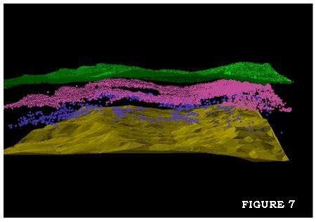
Subtraction of the bare earth values from the canopy layer results in a ‘tree-height’ for merging into a GIS. Current research is demonstrating that multiple return data can be used to derive biomass measurements required for forest inventory, such as, canopy closure, dominant and co-dominant stems, and basal area. Since most of the pulses are at an angle from nadir, the opportunity for a multi-return pulse to strike and penetrate the top (or near the top) of the canopy and continue to record returns with many hitting the ground, is statistically strong. LIDAR is a very consistent sampling technique. Figure 8 is a Canopy Height GIS Coverage derived by subtracting the SEM from the DEM and color-coding the canopy height. The black areas have no vegetative cover; the color values are graduated to the highest canopy (purple).
LIDAR with the proper post-spacing has demonstrated the technology in very dense forests conditions, such as popular tree plantations and riparian vegetation for measuring the canopy height, bare earth, and biomass indicators. Subtle terrain features often unnoticed by forest land managers (abandoned roads, hydrology, geologic features) are often ‘revealed’ by LIDAR terrain mapping.
It is important to note that Northwest forests exhibit a variety of characteristics: canopy closure, stem characteristics, understory components, local environmental conditions, and species type all affect the capacity to accurately determine the desired data. Project planning is of critical importance, and the historical corporate base of knowledge should guide the project design. The complexity and steep areas within each site must also be evaluated for adequate LIDAR point coverages. Having existing imagery and mapping available for project design is required; having current imagery is required to complete the data processing, quality control, and product delivery.
The AeroScan LIDAR System has been developed by the EarthData International Business Group – Spencer B. Gross, Inc. is the NW point of contact.