Readily available GIS data coverages and ArcView GIS were used to explore the possible relationships between water quality in streams and the regional characteristics of the streams' upstream contributing area. This study evaluated the relationships between total phosphorous measurements and the upstream distribution of land use, elevation, and total contributing area. Simple regressions on the data extracted using ArcView GIS were shown to explain a very significant portion of the variation in measurements of total phosphorous in the streams. Study results support the use of regional analysis for prediction of water quality in many applications including development of total maximum daily loads.
One current area of active research in water quality and watershed management is the application of regional characteristics as predictors of water quality in streams. Researchers and regulators are constantly faced with situations in which the water quality of a stream segment is in question but inadequate water quality measurements/data exist to characterize the nature and extent of the water quality problems that could be occurring in that particular stream segment. This is especially true when non-point sources of pollution, which are by nature difficult to quantify, may be the predominant cause of the water quality impairment.
Many researchers have hypothesized that the regional characteristics of the contributing area of streams, including land use, soil type, elevation, relief, agricultural chemical application rates, precipitation, etc., can be used as predictors of the probable water quality in those streams because it is believed that these are the factors that affect water quality. The United States Geological Survey (USGS) has developed one such approach called SPARROW, or SPAtially Referenced Regressions on Watershed Attributes, which relates in-stream water-quality measurements to spatially referenced characteristics of watersheds, including contaminant sources and factors influencing terrestrial and stream transport (USGS, 2000).
Although the idea of relating regional characteristics to water quality has been around for some time, a relatively new concept is to use these possible relationships as a statistical approach to estimate water quality on a single stream system or sub-watershed scale. In cases where these streams have little or no data to characterize water quality, by relating the regional characteristics of the stream's contributing area to the contributing area of streams that have a lot of water quality data, it may be possible to estimate what the water quality would be in the stream that does not have any data.
The utility of a statistical approach to estimating water quality from regional characteristics is that it could fulfill the needs of those in the watershed management community who are faced with a paucity of water quality data and the daunting task of populating parameterized non-point source water quality models with data and information that they simply do not have. A statistical approach may be an excellent way to integrate all available data (from the stream of interest and from streams deemed to have similar regional characteristics) in making an estimate of water quality that would likely be every bit as defensible as one made by one of the more popular parameterized models. A statistical approach to estimating water quality would also fit well as one component in an overall decision support framework for watershed management.
In this report, a simplified, preliminary approach to the regional analysis problem will be presented. As a preliminary exercise, a small subset of water quality predictors was selected for use in predicting a single water quality parameter. In particular, an attempt was made to relate the distribution of land use between agriculture, range land, and forest land upstream of selected water quality control points and the elevation of these control points with the observed levels of total phosphorous measured in the streams at these points. The relation of land use, area, and elevation to total phosphorous was accomplished through generation of the land use/elevation and total phosphorous data using Esri’s ArcView software and geographic information systems (GIS) spatial data contained in EPA’s BASINS (Better Assessment Science Integrating Point and Nonpoint Sources) software, and then by regression analysis of this data in S-Plus, a statistical software produced by MathSoft.
As this was a preliminary study, a discussion of the future work is included in addition to the results. Specifically discussed is how the results of this study will be used, and how a regional analysis approach can support applications that include development of Total Maximum Daily Loads (TMDLs) and watershed decision support.
Relationships between regional characteristics and water quality must be developed and defined through a regional analysis approach, which includes the selection of appropriate water quality predictees (i.e., measurements of the water quality parameters of interest such as total phosphorous, total nitrogen, sediment, etc.), appropriate water quality predictors (i.e., land use data, soil type data, precipitation data, agricultural chemical application rate data, etc.), and the scale and level of detail at which these data are to be used. Total phosphorous was selected as the predictee for this study based on the fact that anthropogenic phosphorous is a very common pollutant in streams. The selection of land use as a predictor was based on the obvious fact that land use affects the amount of phosphorous that enters a stream as non-point source pollution. Control point elevation was added as a predictor in hopes that by including elevation some of the variability in land use with elevation would be captured.
In order to explore the possible relationships between land use, elevation, and total phosphorous concentrations, an adequate source of spatial data had to be selected. The United States Environmental Protection Agency has assembled a multipurpose environmental analysis system for use by regional, state, and local agencies in performing watershed and water-quality-based studies. This software, called BASINS, was developed to facilitate examination of environmental information, to provide an integrated watershed and modeling framework, and to support analysis of point and non-point source pollution management alternatives (USEPA, 2000). BASINS is a tool that integrates environmental data, analytical tools, and modeling programs to support of development of approaches to environmental protection.
A large part of the BASINS software is a GIS database of spatial data that was assembled to support the models and other tools that are included in the package. This GIS database includes national coverages of in-stream water quality data, elevation, and land use/land cover that were utilized in this study to extract the water quality data and elevation at control points and the associated upstream land use data. Table 1 contains a sample of the data that was generated and used in the regression analysis, and the sections following Table 1 describe the process that was used to extract the test data from the BASINS data set so that regression analysis could be performed in S-Plus.
Table 1. Sample of regional analysis data used in regression analysis.
2.1 Selection of Control Points
The BASINS GIS database contains a coverage of water quality monitoring stations that consists of locations at which water quality data has been measured. Since the parameter of interest in this study was total phosphorous, a subset of the water quality monitoring stations coverage was constructed that contains only the water quality monitoring stations at which a reasonable number of measurements (n >10) of total phosphorous exist. A subset of these stations was used as the control points for this study.
Once this coverage of total phosphorous stations was constructed an analysis was conducted to determine whether all of the stream reaches upstream of each control point could be isolated. If it was possible to select all of the upstream reaches, the control point was included in the study. If the upstream reaches were too complicated to isolate or the reach data was incomplete upstream of the control point, the point was left out of the study. It should be noted that the selected watersheds contain mostly low order streams that could be easily isolated. Figure 1 shows an example control point and its associated upstream reaches. This process was repeated until a sufficient number of control points and data were collected for regression analysis. This partial regional data set covers a geographic area that includes a large portion of southeastern Idaho shown in Figure 2.
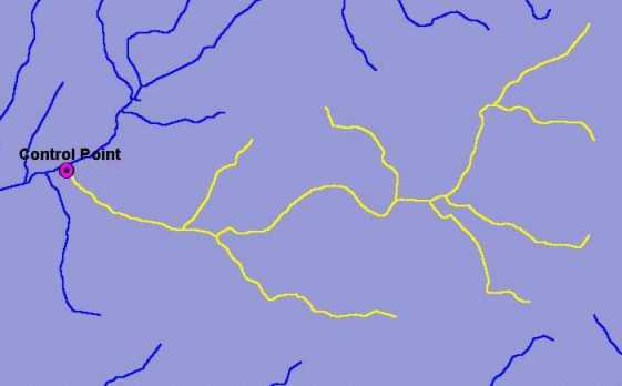
Figure 1. Sample control-point and selected upstream reaches.
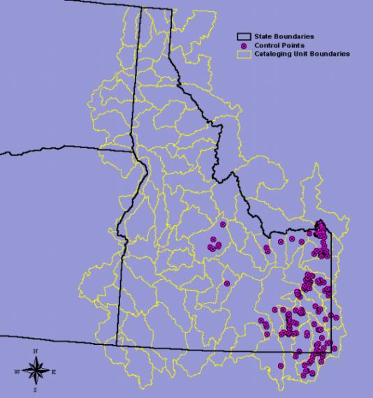
Figure 2. Control Points Used for Regional Analysis.
2.2 Generation of Land Use Distribution Data
Once all of the stream reaches upstream of the control point had been selected, a 100-meter buffer was drawn around all of the selected stream reaches. The 100-meter buffer was used to clip the land use data to produce a land use buffer that describes the land use for a distance of 100 meters on either side of the streams. This technique eliminated the need to go through the complicated process of delineating a sub-watershed boundary for the selected stream reaches and then characterizing the land use distribution in the entire contributing area for the control point (sub-watershed). This simplification was performed based on the assumption that only the land use within 100 meters of the stream really contributes to the concentration of total phosphorous in the stream. In other words, it is assumed that the distribution of land use in the 100-meter buffer around the stream is adequate to describe the relationship between land use and total phosphorous concentrations in the stream at the control point. Limitations of this approach are discussed in Section 6.0 of this paper.
Once the land use buffer had been created, the area in each land use within the buffer was divided by the total area in the buffer to get the percentage distribution for each land use within the buffer. The resulting percentage distribution for each land use within the buffers strongly indicated that agriculture, rangeland, and forestland were the dominant land uses for the data set we considered. Very few, if any, of the control points selected had any other significant land use categories other than these three. For this reason, agriculture, rangeland, and forestland were selected as the three land use categories for regression analysis. Figure 3 shows the land use buffer associated with the selected stream reaches shown in Figure 1.
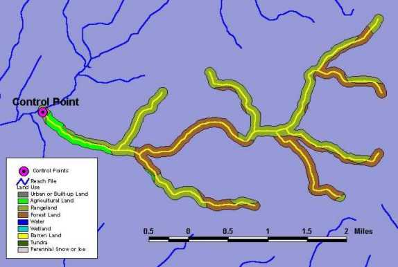
Figure 3. Land use buffer used to calculate percent distribution of land use.
2.3 Elevation Data
The BASINS data set also contains a coverage of elevations for the geographic area that was used in this regional analysis. This coverage was used to pick off the elevation of each of the control points, and the extracted elevation data was added to the land use distribution data. The elevation of each of the control points was added in an attempt to capture some of the variation in total phosphorous that may be attributed to differences in the other variables caused by elevation. For example, agriculture and rangeland at an elevation of 1000 meters is most likely very different than the agriculture and rangeland that could be found at an elevation of 2000 meters. The land use data that was used does not make any distinctions between the types of agriculture or rangeland that may exist in each of these general categories.
Since the purpose of this study was to relate water quality at a control point to the regional characteristics of the upstream contributing area, a simple linear model was constructed with the total phosphorous concentration as the predictee and the five variables in Table 1 (percent agriculture, percent rangeland, percent forestland, total area, and control point elevation) as the predictors. To do this, the effects of each of the chosen predictors (main effects) and all of the possible combinations of the predictors (interactions) on the total phosphorous concentration were explored.
A relatively simple method called stepwise linear regression was used to explore the effects of each of the main effects and interactions between variables on the total phosphorous concentration. With five variables the possibility existed of having a fairly large number of main effects and interactions as terms in the linear model equation. It was also likely that only a select few of these terms would be statistically significant in predicting the total phosphorous concentration. Using the stepwise linear regression approach in S-Plus, it was possible to start with a model that included all of the main effects and interactions (all variable combinations) and then drop terms based on whether they significantly improve the model or not.
The stepwise linear regression routine in S-Plus uses what is called a Cp statistic to determine whether a model is improved by dropping a term. The routine starts with the given model (all main effects and all interactions) and returns an ANOVA table that shows the effects of dropping in turn each term from the model. The columns returned in the ANOVA table show the degrees of freedom for each deleted term, the sum of squares corresponding to the deleted term, the residual sum of squares from the resulting model, and the Cp statistic for the terms in the reduced model. If any term has a Cp statistic lower than that of the current model, the term with the lowest Cp statistic is dropped (MathSoft, 1997). If the current model has the lowest Cp statistic, the model is not improved by dropping any more terms. The result of the stepwise linear regression process was a linear model predicting the total phosphorous concentration and containing the minimum number of terms (variables and combinations of variables) that are found to be significant.
Once a model had been produced, several diagnostics were examined to determine how well the model fit the data. First, the multiple R2 value for the model was examined to see how much of the total variation in the data was explained by the model. Second, several diagnostic plots were made to help in determining how well the model fit the data. Comparison of the R2 values and the diagnostic plots for the models produced helped in deciding whether transformations of the data would be helpful, and then finally in deciding which model was the best at predicting the total phosphorous concentration using the given predictors.
Stepwise linear regression on the regional analysis data produced a linear model with a relatively poor R2 value (=0.40). The low R2 value means that only approximately 40 percent of the variability in the mean total phosphorous data is explained by the model produced. The diagnostic plots for the regression on the regional analysis data identified some inherent weaknesses in the model including non-constant variance in the residuals produced by the model and residuals that were not normally distributed. The diagnostic plots did, however, suggest that transformation of the data may improve the model.
Log-transformation of the mean total phosphorous data significantly improved the R2 value to approximately 0.62. The diagnostic plots for the regression on the log-transformed data showed that after log-transformation the regression produced constant variance in the residuals produced by the model. The residuals also appeared to be normally distributed, which is characteristic of a good model. Although the residuals appeared to be normally distributed and have constant variance, a plot of the spread of the residuals versus the spread of the fitted values (a standard residual fit spread plot in S-Plus) showed that the spread on the residuals was nearly as great as the spread of the fitted values. Since the object of the model is to explain the variability in the mean total phosphorous data it is hoped that the degree of spread of the residuals be much less than the degree of spread of the fitted values (MathSoft, 1997). Therefore, this is an apparent weakness in the model produced by log-transformation of the mean total phosphorous data.
Further analysis of the diagnostic plots showed that several "extreme" values were affecting the model to a much greater degree than any of the other values. This was the reason behind the weakness in the model identified above. After removal of the identified "extreme" values, the R2 value for the model improved to approximately 0.83 and the spread on the residuals was also significantly improved. The model showed that the most important variables are percent agriculture, percent forest, percent rangeland, elevation, and the combined effect of agriculuture and rangeland, and agriculture and forest. It is interesting to note that the total area in the buffer was not significant in the model produced. The following are the important diagnostic plots for the model, and following each figure is a discussion of its significance.
Figure 4. Residuals versus fitted values for data set with extreme values removed.
The plot of the residuals against the fitted values (Figure 4) is designed to reveal any unexplained structure left in the residuals, which in a strong model should appear as nothing but noise. In a model that fits the data well, the residuals would appear to be normally distributed about zero (the mean of the residuals would be zero). Figure 4 shows that the residuals for this model appear to be randomly distributed about zero with no apparent trends.
Figure 5. Normal quantile plot of residuals for data with extreme values removed.
Figure 5 is designed to provide a visual test of whether a model’s residuals are normally distributed. If the ordered residuals cluster along the superimposed quantile-quantile line, there is strong evidence that the errors are indeed normal. Figure 5 shows that most of the residuals are clustered along the superimposed quantile-quantile line, giving little reason to conclude that the residuals are not normally distributed. This evidence also supports the significance of the model with extreme values removed.
Figure 6. Residual fit spread plot for data with extreme values removed.
The residual fit spread plot is designed to compare the spread in the residuals with the spread in the fitted values. Since the object is to explain the variation of the data, the spread on the residuals should be less than the spread on the fitted values. Figure 6 shows that the desired result has been achieved with this model.
Figure 7. Log of mean total phosphorous versus fitted values for data with extreme values removed.
This plot gives an idea about how well the model has captured the broad outlines of the data, and for a well-fitted data set the data points should be close to the diagonal line. The better the model fits the data, the less the spread about the diagonal line.
The results of the stepwise linear regressions done in this study show that a very significant amount of the variability in the measurements of total phosphorous at control points can be explained using a simple linear model that includes land use, total area, and elevation as predictors. The R2 values for these regressions ranged from about 0.4 for the model produced from the untransformed data to approximately 0.8 for the model produced from the transformed data with the extreme values removed. The diagnostics for the models with higher R2 values appear to support this conclusion.
The various model runs in this study showed that log transformation of the data produced better regression results. The regression results were also very significantly improved by removing several of the extreme values in the data that influenced the regression the most – as identified in the diagnostic plots for the individual models.
It can be concluded that the most important variables in predicting the mean total phosphorous concentrations were percent agriculture, percent forest, percent rangeland, elevation, the combined effects of percent agriculture and percent rangeland, and percent agriculture and percent forest. Total area, although significant in some cases, did not have a significant model coefficient in the model that was judged to be best by the analyses. The Model Output for log-Transformed Total Phosphorous Versus Untransformed Percent Agriculture, Rangeland, Forestland, and Elevation after Removal of Extreme Values was considered the best (R2 = 0.83).
Overall, it appears that the results of this study support the theory that water quality at control points can be predicted using regional characteristics of the upstream contributing area. This study showed that a very significant amount of the variation in the measurements of one water quality parameter (total phosphorous) could be explained by a simple linear regression that included only land use, contributing area, and elevation as predictees. It is very possible that if additional predictees were included in the regression (i.e., soil characteristics, average precipitation, relief, agricultural chemical application rates, etc.) the result would be a higher R2 value and a model that is much better at predicting the total phosphorous concentration. It may also be possible to do a similar study for other water quality parameters such as sediment or dissolved oxygen to see whether similar relationships between regional characteristics and water quality parameters could be developed.
This study shows a clear relationship between in-stream total phosphorous and the selected set of watershed attributes. More importantly, it demonstrates the potential utility of statistical and data driven approaches for estimating water quality. Future work in this area will include addressing the following deficiencies in the current approach:
Modeling units: In this study, modeling units were chosen as the region of land surrounding all stream segments upstream of a given control point within a 100-meter buffer. This was done under the assumption that the effects of land processes immediately adjacent to the stream segments are more dominant than processes further away from the stream. This assumption may be valid in many cases but does not allow for inconsistent stream digitization. By not accounting for these inconsistencies, the resulting models are biased towards streams that were more thoroughly digitized. In future work, we intend to address this problem by not using 100-meter buffer strips as modeling units. Instead, we will use the entire contributing area to the control point as defined by a watershed delineated from elevation data.
Water quality data: The water quality data presented in this study was limited to total phosphorous measurements extracted from water quality summaries included in EPA's BASINS data sets. These summaries do not account for temporal variation in the data and as such may not be appropriately comparable. Current and future efforts to improve the methodology presented here will utilize raw water quality observation at the selected control points. By using the raw data instead of summaries, we will be able to build unique models for different seasons.
Predictor data: This study used a very limited predictor set including land use, elevation and contributing area. While these predictors did show strong relationships with the predicted water quality data, a larger set of predictors may perform even better. Future efforts in this area will use additional predictors such as soil and climate data, census information, county fertilizer and pesticide records and additional physical and geomorphologic information.
Methodology: The purpose of the study discussed above was merely to explore the possibility of whether significant relationships exist between water quality in streams and the regional characteristics of the upstream contributing area. The linear regressions presented in this paper were meant only to show that there is evidence that a statistical water quality model may be useful. Once it is established that these relationships exist, however, the question becomes how to use these relationships in a useful way. Current plans for improving this methodology include using nonparametric methods and Bayesian networks to estimate the relationships between the predictor set and the selected water quality parameters. Such methodologies will ultimately allow this regional regression approach to be tied into a larger decision-making framework based on Bayesian networks currently under development at Utah State University.
Berthouex, P.M. Brown, L.C. 1994. Statistics for Environmental Engineers. Lewis Publishers. Boca Raton, New York.
MathSoft, Inc. 1997. S-Plus Guide to Statistics. Data Analysis Products Division. MathSoft, Seattle.
USEPA. 2000. BASINS 2.0 Fact Sheet - A Powerful Tool for Managing Watersheds. http://www.epa.gov/OST/BASINS/basinsv2.htm
USGS. 2000. SPARROW-SPAtially Referenced Regressions On Watershed Attributes for Modeling of Surface-Water Quality.http://water.usgs.gov/nawqa/sparrow/index.html