Abstract

The integration of social and natural science data is part of CIESIN's mission to help scientists, decision-makers and the public gain a better understanding of their changing world. Information on global human population is collected by administrative units that are poorly suited for integration with natural science data, which are often collected on a grid. CIESIN, The International Food Policy Research Institute and the World Resources Institute have collected sub-national administrative and population data and produced a grid of global population at a resolution of 2.5 arc minutes. This paper showcases the gridded product; addresses conceptual, methodological and technical issues in the production of the grid; and discusses issues of input data quality.

Introduction

Demographic information is often provided on a national basis, but global environmental and other cross-disciplinary studies usually require data that are referenced by geographic coordinates, such as latitude and longitude, rather than by political or administrative units. During a 1994 workshop on Global Demography, a consensus was reached that a consistent global database of population totals in raster format would be valuable for interdisciplinary study. This consensus resulted in the development of the first version of Gridded Population of the World, which was released in 1995 (Tobler et al., 1995).

Version 2 of the Gridded Population of the World (GPW) data set has been developed by the Center for International Earth Science Information Network (CIESIN), the International Food Policy Research Institute (IFPRI), and the World Resources Institute (WRI) to aid in the integration of social and natural science data. 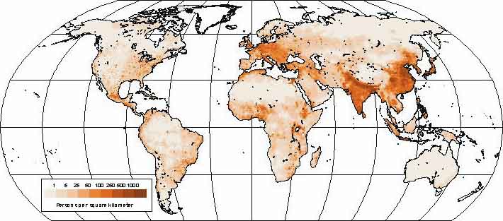In both versions of GPW, the distribution of human population is converted from national or sub-national units to a series of georeferenced quadrilateral grids. Version 2 of GPW uses improved input data and a revised gridding methodology to produce a global grid of the distribution of human population at a resolution of 2.5 arc minutes.  A projected, reduced resolution image of the final GPW product is shown in Figure 1.
 

Figure 1. Global population density, 1995 adjusted data.
Detailed images and the data for GPW version 2 are available at:
http://sedac.ciesin.org/plue/gpw

Overview

The general steps for producing version 2 of GPW are listed below.  The specifics of the methodology and the issues that arose related to these steps are described in later sections. ArcInfo^TM was used for processing in all of the steps except the last one and the subsequent merging of the grids, which were completed in GRID^TM. For each country or area, the following steps were carried out:

• Obtain digital administrative boundaries and population data.
• Reconcile boundaries with neighboring countries and improve coastlines where necessary.
• Estimate 1990 and 1995 population by administrative district (P90 and P95) and add the population data to the digital administrative map.
• Calculate a national level adjustment factor by comparing population estimates and the United Nations Populations Prospects (United Nations, 1999) estimate of total population.
• Create alternative population estimates for 1990 and 1995 (P90A and P95A) by applying the adjustment factor calculated in step 4 to each administrative unit so that the national total matches the United Nations World Population Prospects estimate.
• Overlay a digital map of lakes and ice covered areas and set the population estimate for these areas to zero.
• Compute population densities (now net of lake and ice areas) for each administrative unit in square kilometers.
• Union an empty vector format grid (fishnet) at a resolution of 2.5 arc minutes with the input administrative data.
• Calculate the area in square kilometers for each polygon in the "unioned " coverage, and multiply this area with the population density of the corresponding administrative unit to get a population estimate for each polygon of overlap.
• Aggregate the four population estimates and the land area in square kilometers for all polygons of overlap that belong to a given grid cell and link these grid cell totals back to the original regular grid (fishnet).
• Convert this result to five raster grids: one each for population in 1990 and 1995, adjusted and unadjusted, and one for land area.

Source Data

Geographic Information System (GIS) data sets of administrative or statistical reporting units are produced by national statistical and mapping agencies, research projects, and commercial data vendors. Data for GPW were obtained from over 40 different suppliers.  Improved data for Africa, Asia and Latin America were obtained from non-commercial sources. Additional boundary data sets - for Europe, Canada, Australia/New Zealand, India, Malaysia, and the newly independent states of the former Soviet Union - were obtained from commercial data vendors. The boundary data sources for each country are available as part of the GPW web service (see the documentation portion of the service available at: http://sedac.ciesin.org/plue/gpw/ for details).

In total, we assembled boundaries for more than 125,000 administrative units, about 60,000 of these units being census tracts in the United States. Even without the very detailed information for the USA, however, the database provides significantly higher resolution than the previous version of GPW, which was based on about 15,000 units. The spatial resolution of the boundary data varies by country. A summary of the administrative levels obtained is shown in Table 1.
 

Table 1. Summary of Administrative Levels

Administrative Level	Frequency	Cumulative Percent	U.S. Equivalent
0	47	22.2	Nation
1	68	51.8	State
2	88	91.4	County
3	18	99.6	Tract
4	1	100.0	Block
Total	222	100.0

Source Data Preprocessing

To ensure consistency at international borders, most national boundaries in the source data were replaced by the political boundaries from the Digital Chart of the World (DCW) (NIMA, 1993). Where the DCW contains more detailed coastlines, the administrative boundary data coastlines were also replaced with the DCW data. While not perfect, DCW data are the most widely used template for global and continental GIS studies. Exceptions where international boundaries were not replaced include parts of Europe and North America, which already had matching international boundaries, and any countries for which the boundaries have changed since DCW was issued.

Population estimates for the administrative units were adjusted to match the two reference years (1990 and 1995) using standard demographic techniques.  Adjustment factors were also calculated based on the difference between national-level population totals from census or other data sources and the estimated national population figures published by the United Nations (UN) in Populations Prospects (United Nations, 1999).  This adjustment factor was used in the gridding processing to derive grids that match the UN population totals.

Issues in Source Data Collection and Use

Gridding the source administrative data is advantageous for a number of uses (e.g., modeling, integration with data collected on different units).  However, providing population data on a grid is also the only way in which all of the data collected could be distributed freely for scientific purposes.  An integrated, sub-national boundary data set for the world, such as the one developed for GPW, would be a useful data set. Unfortunately, government and commercial vendor copyright restrictions on a number of the input data sources prevents the distribution of this data collection.

As with any global data set collected from various sources, the quality of both the population estimates and spatial boundaries in the source data varies.  This variability affects the quality of the final grids in GPW.  While the population estimates collected for GPW vary in quality, the data collected represent the best available that could be obtained for each country. The GPW methodology is designed so that updates of individual countries can be incorporated without the need to re-process all of the data.  This will allow future improved population estimates and boundary data to be incorporated into the regular updates planned for the data set.

In countries where there has not been a recent census, the population estimates are outdated (e.g., Afghanistan, Albania).  This results in a long extrapolation period to estimate the population in the reference years, which increases the uncertainty in the estimation. Unfortunately, until a new census is undertaken in these countries there is no simple remedy for this problem. Similarly, there is no ready solution for countries that only had sub-national population estimates for one date.  National level growth rates had to be used to produce the sub-national 1990 and 1995 estimates for these countries. As of result of using national level estimates, sub-national variation in population change is masked in the final product.

Where significant population displacement since the last enumeration has occurred, the population estimates are inaccurate (e.g., former Yugoslavia, Rwanda-Uganda). Care must be taken when data from these areas are used for analysis. In certain cases, the population estimates obtained from national or other agencies vary significantly from those published by the UN (e.g., Somalia, Paraguay). Methodological differences, political policies, and the time lag between national estimation and UN estimates may be responsible for these variations. Data adjusted to match the UN estimates is also provided because the UN estimates often reflect adjustments of nationally reported figures to compensate for over- or under-reporting. Unfortunately, the UN estimates are only available at the national level. Sub-national variation in the adjusted grids does not reflect the adjusted data provided by the UN, all of the administrative units were adjusted uniformly.

The spatial data used in GPW are also of variable quality.  Many of the data sets were of uncertain quality with regards to the source of the boundaries, original scale and level of generalization. When multiple data sets were available, we always opted for higher resolution (more administrative units), which for a global application is considered more important than high positional accuracy. In some instances, the spatial boundaries did not exactly match the reported administrative units. In these cases we had to use judgment to assign population totals to digital administrative units.

Gridding Methodology

The input data on administrative unit boundaries and population totals were used to produce raster grids showing the estimated number of people residing in each grid cell. In contrast to previous efforts, we did not distribute population within each administrative unit - either on the basis of proximity to large towns, infrastructure and other factors influencing population distribution (as in the Africa, Asia and Russia data sets); or based on a smoothing method that assumes that grid cells close to administrative units with higher population density tend to contain more people than those close to low density units. The second option was implemented using a smooth pycnophylactic interpolation in version 1 of GPW (Tobler et al. 1995, 1997). The new raster grids are thus similar to the unsmoothed grids of version 1 of GPW. The cell size for the new population grids is 2.5 arc minutes, or about 5 km at the equator. Figure 2 below illustrates the cell size in relation to the administrative units for the Dominican Republic. The cell outlined in blue is used to illustrate the gridding approach in more detail, as shown in Figure 3.

Figure 2. Grid cell size in relationship to administrative boundaries, Dominican Republic.

In contrast to the unsmoothed grids for version 1 of GPW, we used a different gridding approach for this update. In version 1 a standard GIS polygon-to-grid conversion function was used. This function assigned a grid cell to a specific polygon based on a simple majority rule. This has a number of disadvantages: grid cells that contain parts of several administrative units are assigned to only one unit, and units that are smaller than the cell size may be lost. To prevent these problems, we used a proportional allocation of population from administrative units to grid cells. That means that - assuming constant population densities in a unit - if five percent of an administrative unit falls within a given grid cell, five percent of the unit's population will be assigned to it. This method of interpolating data between incompatible reference units is sometimes called areal weighting.

The assumption of uniform distribution of population is not an accurate model of human population distribution over administrative units. People tend to reside in clusters of varying density, and the remaining parts of administrative units are typically less densely populated or empty. Uniform distribution and areal weighting were chosen for several reasons:
 

• This type of model required no ancillary data for distributing the population.
• The single variable model can be used for analysis with other data sets not based on administrative data without raising concerns about false correlations or conclusions (the two are independent).
• Variations in population at large scales are less important for global and regional studies for which GPW is considered appropriate.
• The use of a simple model of population distribution, in which the assumptions are all known, simplifies the interpretation of the results of analysis.

Figure 3. Detail of gridding approach for cells containing boundaries
 
 

Table 2. Areal weighting scheme to allocate population over multiple grid cells

Administrative Unit Name	Admin Unit Density (persons/sq km)	Area of Overlap (sq km)	Pop Estimates for Grid Cell
Santiago Rodriguez	64.2	5.3	340
Santiago	246.5	2.2	543
San juan	75.9	12.8	972
Total for Cell	91.3	20.3	1854

Since larger water bodies can significantly distort the actual population density within administrative units, we used a mask (or filter) consisting of the larger lakes and ice covered areas in the DCW. We implemented this gridding routine for each country individually and later merged the national grids to produce continental and global raster data sets of population counts (number of people residing in each grid cell). Population grids for 1990 and 1995 - both unadjusted and adjusted to match the UN estimates, are available for the global, continental, and country coverages. In addition, the 2.5 arc minute grids have been aggregated to produce high quality coarser grids, for use in applications, such as climate modeling, which require data aggregated to 0.5 or 1.0 degree grid cell.

Since the grids use the latitude/longitude reference system, the actual size of a grid cell in square kilometers varies as a function of latitude, with a maximum cell size of about 21 square kilometers at the equator. We therefore produced a fifth grid which shows the total land area in each grid cell. This is actually the grid cell area net of water bodies (lakes and ice or oceans). Dividing the grids of population counts by the area grid yields population density grids that can be used for mapping and analysis. Figure 4 shows a population density at 2.5 arc minute resolution for Haiti.

Figure 4. Population density for Haiti at 2.5 arc minutes.

For grid cells in bordering lakes or oceans, the cell's land area can be considerably smaller than  neighboring cells that are completely on land. Cartographically, this means that grid cells of population density will be shaded completely, even if only a small portion of the cell is covered by land. For instance, Figure 5 shows grid cells and administrative units for a small area in the north of Haiti including the Ile de la Tortue.

Figure 5. Population density and administrative boundaries for a portion of Haiti.

As an example, the cell in the center of the top row has a land area value of only 0.97 square km. With a population density of 286.7, 278 persons are assigned to that cell. The cell immediately below, with a land area of 20.14 and the same density, contains an estimated 5774 people. This approach thus exaggerates the land area of a country in cartographic displays (however, grid cells with small land areas can be masked easily for mapping using a threshold applied to the area grid). Yet computations using these grids are more exact than computations that utilize a standard GIS provided polygon-to-grid routine in which grid cells that are located in coastal areas would be completely allocated to either land or water areas.

Issues in Methodology

The assumption of uniform distribution over an administrative unit (as discussed above) is not an ideal model of human population distribution. Other models, such as the one used by Dobson, et al. (1999) in the creation of the Landscan database, are possible; however, they would require ancillary data and the results would not have the advantages of a single-variable model. It is possible to combine the GPW population grids with other data, perhaps even another gridded population data set, to produce a combined population surface that suits a particular study or application.

Resolution varies greatly between countries, which is reflected in the merged grids. Since the gridding algorithm is applied to individual countries and the results are summed to produce the global grids, updating one or many countries is simple. We plan to update GPW on a periodic basis, these updates will include any improved boundary or population estimates that are obtained.

The production of population estimates for two dates complicates the task of matching population estimates to spatial units due to boundary changes over time. One set of boundaries was used for both reference years in version two of GPW.  This resulted in several instances where population redistribution had to be done because of boundary changes.  This process is not overly complex for only two dates. However, as more estimates become available and the data are revised, tracking changes and maintaining consistency the links between boundaries and population estimates becomes both crucial and a more complex task.

The production of quadrilateral grids rather than a grid with uniform resolution can complicate the use of the data for some applications. For example, the integration of GPW with projected data requires that one of the data sets be transformed so that it will match (spatially) the other data sets being used.  If GPW is transformed, interpolation of the grid cell values between the original raster array and the output grid is required. This can introduce error in the attribute data and affect regional population totals. Producing GPW on an equal-area grid would not remove the need for transformation in many cases, since there are many different global projections, each with their own advantages and drawbacks. A geographic grid was chosen, as it is a standard, easily transformed coordinate system.

References

Dobson, J. E., E. A. Bright, P. R. Coleman, R. C. Durfee, and B. A. Worley, 2000.  "A Global Poulation Database for Estimating Population at Risk," Photogrammetric Engineering & Remote Sensing, 66(7).

[NIMA] National Imagery and Mapping Agency, 1993.  Digital Chart of the World, downloaded from: Pennsylvania University Libraries (http://ortelius.maproom.psu.edu/dcw/).

Tobler, W., U. Deichmann, J. Gottsegen and K. Maloy (1995), The global demography project, Technical Report 95-6, National Center for Geographic Information and Analysis, Santa Barbara.

Tobler, W., U. Deichmann, J. Gottsegen and K. Maloy. 1997. "World Population in a Grid of Spherical Quadrilaterals," International Journal of Population Geography, 3:203-225.

United Nations, 1999. World Population Prospects: The 1998 Revision. Volume 1: Comprehensive Tables.  NY: United Nations.

Author Affiliations

Gregory Yetman: CIESIN, Columbia University

Uwe Deichmann: The World Bank

Deborah Balk: CIESIN, Columbia University