A Decision Support System for Enhancing Model Development and Application
Fernando Toro and Roberto Mayerle
Abstract:
This paper presents a Decision Support System (DSS) developed for enhancing numerical model development and applications in rivers, estuaries and coastal areas. The DSS is to speed-up data analysis through a GIS user-friendly interface by adequately storing, managing and integrating in-situ measurement data and model results and allowing for the possibility of exporting the results directly to reports. It has been tailored to the Delft3D Flow Module outputs and focuses primarily on measurement data on water levels from gauges and current velocities from ship mounted and stationary Acoustic Doppler Current Profilers (ADCP) from RDI Corporation. In this paper the system is described and its application in the calibration of a two-dimensional depth integrated model for simulating the processes in a tidal flat region in Northern Germany are shown.
1. Introduction
During the last decade significant advances have been made in the numerical modeling field and in the development of measuring devices for rivers, estuaries and coastal areas. As a result, simulations of real world problems (large domains and fine grid systems with millions of nodes) with high degree of accuracy in conjunction with field measurement data have been carried out successfully.
Model development and application requires a huge amount of handling of in-situ measurement data and model results. Nowadays, a significant percentage of time (with respect to the total time) is required for preparing, analyzing, integrating measurement data and model results as well as in taking decisions regarding for example the optimum model settings and best solutions to the problem in question. Since these data sets are quite inhomogeneous (e.g. continuous measurements of point information and area measurements at irregular time intervals), distinct analytical tools are required to handle each data type. While, in general, they are very efficient in dealing with a specific data type and particular tasks, there is a lack of systems creating a common working environment to effectively cover the whole spectrum. Besides, only a limited number of systems are capable of adequately integrating in-situ measurement data and model results and only a few of them enable the output of the results of the analysis directly into reports. Since a significant amount of the time is spent in handling the data, there is a need for tools that support the modeler in the development and application of the model.
In this paper a Decision Support System (DSS) under development at the Coastal Research Laboratory of the University of Kiel in Germany is presented. It aims at speeding-up data analysis, and enhancing model development and application through a user-friendly interface by adequately storing, managing and integrating in-situ measurement data and model results and allowing for the possibility of exporting the results directly to reports. An application of the DSS in conjunction with the development of a model of a tidal flat area along the German North Sea coast is presented herein.
2. The Decision Support System
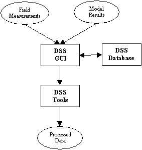
The main components of the DSS are sketched in Figure 1. It comprises a Graphical User Interface (GUI), a database and several tools that have been built on the basis of ArcView® V.3.2 (Esri, 1996a), Matlab® V.6.0 (The Math Works, 2000), Visual Basic® V.6.0 (Microsoft, 1999), C++ and MS Excel® (Microsoft, 1997).
Figure 1: Components of the DSS
Field measurement data and model results (water levels and current velocities) are imported to the DSS via GUI. Tools that have been developed for formatting (standard format) and correcting the data can be used. A database is created during the data import. Data are imported using the GUI in an automatic fashion through GIS software, giving the possibility to display in a map the areas where available data are and select data for plots and comparisons.
Linking model and field measurements to GIS and a database management system can facilitate better data storage, manipulation and analysis than conventional methods. Thereby, it reduces the time required to analyze the numerical model outputs and enables users to identify critical areas and perform various "what if" scenarios to support the decision-making processes.
Once the data are imported in the DSS, visualisation tools allow the modeller to compare model and field measurements, prepare plots and carry out statistical analysis.
The system facilitates model development tasks by enabling measured data and model results to be displayed and processed thereby helping the model developer to make comparisons and thus taking decisions regarding the optimum model settings. It is to be used for model development (sensitivity analysis, calibration, validation and application) and on-board during measuring campaigns for displaying and analysing measured current velocities from ship mounted ADCP and integrating them directly with results of model simulations carried out in real time thus enhancing the cost-effectiveness of such activities.
Data sources and file formats: The DSS has been tailored to the Delft3D Flow Module developed at WL Delft Hydraulics, the Netherlands (WL Delft Hydraulics, 1999), and focuses primarily on measurement data on water levels from gauges and current velocities from ship mounted and stationary Acoustic Doppler Current Profilers (ADCP) from RDI Corporation (RD Instruments, 1994).
Delft3D is a multidimensional (depth-integrated-2DH and three-dimensional-3D) simulation program. In the 2DH mode, water levels and depth-integrated velocities (magnitude and direction) at every nodal point are computed on a horizontal grid. The 3D Flow Module computes in addition to the water levels, three velocity components at every nodal point on a three dimensional grid. Throughout the domain, a variable number of nodes can be considered over the depth. The results are stored in binary format files covering the entire domain and simulated period. These files are read with DSS tools and converted in ASCII files for the location and period the modeller requests.
Water level measurements are usually available as time series at several locations and provided in ASCII format. Moored ADCP provides time series of the velocity distribution (magnitude and direction) over the depth at fixed time intervals (Ensembles) and vertical layers (BINs); whereas data from ship mounted ADCP gather velocity distributions (magnitude and directions) over the depth along ship tracks (ADCP transects) at fixed distance intervals (Ensembles) and vertical layers (BINs). The measured data is converted into an ASCII format for further use before importing it in the DSS.
Figure 2 shows typical sketches of data recordings and outputs from ADCP devices used at a) a fixed location in which recordings are in a time series with water levels changing according to the tidal cycle and b) as ship mounted device with location changing along the ship path (ADCP Transect).
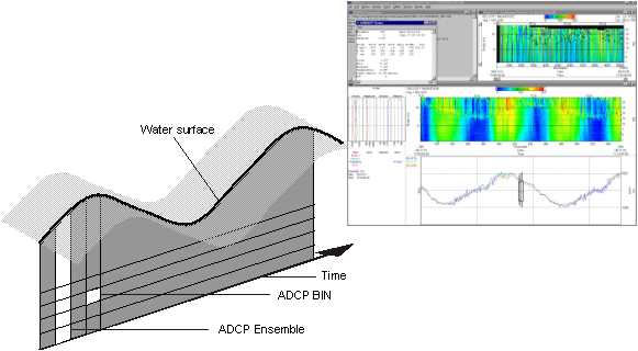
a) Moored ADCP
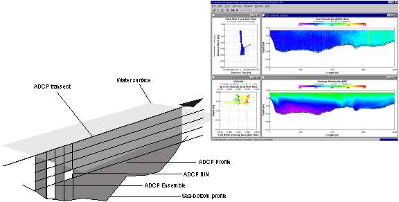
b) ADCP profile from ship mounted device
Figure 2: Typical outputs from ADCP
Graphical User Interface (GUI): The GUI is responsible for integrating the various system components and data sources. It uses the ArcView environment, and it is customized using AvenueTM (Esri, 1996b) allowing the user to navigate efficiently using "point and click" methods. Executing the import of data and other tasks automatically reduces the amount of information to be handled. The DSS simplifies the procedure of data entry by providing a simple and flexible graphical interface. Within the GUI, a map of the research area showing the available data and its location gives an overview about the existing data. Other components of the system can be assessed from here and several of the tasks can be performed with the data. In addition to the tools developed at Corelab, the GUI benefits from all the tools and capabilities of the ArcView software such as legend customization, labels, drawing tools, zooms and map layouts.
Database: The management of the data is performed using the ArcView-GIS software in conjunction with a relational database system. A relational database is a collection of data items organized as a set of formally described tables from which the data can be accessed or reassembled in many different ways without having to reorganize the database tables. In addition to being relatively easy to create and access, relational databases can be easily extended. Once the data is entered, the necessary tables are automatically created and relationships between the input data and the system database are established. Due to the amount and type of data to be handled, the management of the data files that support the database is carried out in the form of a directory tree structure with data measurement, model result and the DSS output subdirectories. New directories and files are created inside a case directory to store data from user inputs and system outputs. The DSS maintains a tight control of all data, location of files and relationships among the data sets. The database is queried, and the retrieved data is analyzed to present the results in the form of maps, tables and plots tailored to handle model results and in-situ measurements.
Source file names, location, date, time and magnitudes of the measurements are stored in the database tables gathered in three main groups according to the data source, i.e., water levels, current velocities and model results.
Tools: In addition to the handling of various tedious and error-prone tasks, several software tools have been developed and are implemented in the DSS. These include a collection of tools for: 1) data processing before entering the DSS; 2) data import; 3) data visualization; 4) statistical analysis; and 5) exporting the results of the various analyses directly into reports.
Pre-processing: Several tasks have to be performed with the data before it is imported to the DSS. These include changes to a standard data format, pre-defined reference levels along the vertical (the German Normal Null is used as the reference level along the vertical) and horizontal directions (projection of geographic coordinates onto a plane) and with respect to time reference (all the data is referred to the UTC, i.e. Coordinated Universal Time). Such tools have been programmed using Matlab, Visual Basic, C++, MS Excel macros and Fortran. They are stand-alone subroutines that can be used from the GUI and also run separately having a user-friendly interface.
Data import: Data from field measurements and model results are saved respectively in the measurements and model directories within the DSS directory tree structure. Measurement data (water levels and current velocities) is converted to ASCII format to be used within the DSS. This data is handled with the help of Avenue scripts, which have been tailored to read ASCII files (in various formats) directly into ArcView tables. The projection of the locations at which measurements were carried out for positioning the data in the study area is done with the help of CVGK and GK V.2.1 software developed by Rathlev, 1998. Model results are stored as files in binary format. Since these files are usually large and only part of the information (in space and time) is needed, the Viewer Selector V1.10 developed by Delft Hydraulics (Delft Hydraulics, 1997) is used. It is integrated within the DSS and enables the user to select the required information and to save it in ASCII format for further use.
Visualization: Data visualization is done entirely with ArcView and Matlab software. Several tools have been developed for preparing plots comparing measurement data, model results and a combination of them. Table 1 summarizes the plots supported by the DSS to handle data on water levels and velocities as point information, velocities along ship tracks (cross-sections or longitudinal profiles) from ship mounted ADCP and velocity fields covering a certain area in conjunction with 2DH and 3D Flow Modules. Figures 6, 7 and 8 from the next section (Application of the DSS) show examples of plots used to visualize respectively point information, information over cross-sections and information covering a certain area. To allow for direct comparisons with the 2DH model results, the measured current velocities are integrated over the depth.
Table 1: Plots supported by the DSS
|
2DH Model |
3D Model |
|
|
Point information (water levels and velocities from moored ADCP) |
Time series of water levels |
Time series of water levels |
|
Time series of depth integrated velocities |
Time series of velocities at a given location (or the corresponding depth integrated value) |
|
|
Time series of a combination of water levels and depth integrated velocities |
Time series of a combination of water levels and velocities at a given location (or the corresponding depth integrated value) |
|
|
Vertical velocity profile at a given location and time |
||
|
Information over cross-sections or longitudinal profiles (velocities from ship mounted ADCP) |
Depth-integrated velocities for a given time |
Velocities at a certain depth and percentages of depth (or the corresponding depth integrated value) for a given time |
|
Cross-sectional averaged velocity (or flow discharge) covering a certain period |
Cross-sectional averaged velocity (or flow discharge) covering a certain period |
|
|
Isovels of velocity over the depth for a given time |
||
|
Isovels of depth-integrated velocities over the ship track covering a certain period |
Isovels of the velocities at a certain depth and percentages of depth (or the corresponding depth-integrated values) over the ship track covering a certain period |
|
|
Information covering a certain area (velocities from ship mounted ADCP) |
Vector field of depth integrated velocities |
Vector field of velocities at a certain depth and a given percentage of the depth (or depth-integrated velocity field) |
Statistical analysis: Tools for carrying out statistical analysis on measured data, model results and a combination of them have been implemented in the DSS. These also include the analysis of the discrepancies between model results and measurement data during the calibration and validation of the model.
Output into reports: During model development and application a large number of plots and tables analyzing and comparing field data and model results are prepared. Since they need to be included in a report. Processes to produce several plots (in batch mode) have been automated and can be exported directly onto formatted sheets to be included in reports.
3. Application of the DSS
An example of the application of the system in the calibration of a 2DH model is presented hereafter.
Investigation area and project: The area of investigation is the Meldorf Bay and the adjacent tidal channels on the German North Sea coast. It covers an area of about 400km2. The results presented are part of the research project "Predictions of Medium Scale Morphodynamics-Promorph" (Zielke et al., 2000) funded by the German Ministry of Education and Research from 2000 to 2002. The aim of the project is to develop, calibrate, validate and apply numerical models to the simulation of morphological changes over periods of several years. The tidal channels have a maximum depth of about 20m. Tidal range is around 3.0 to 3.5m. Figure 3 shows the location of the investigation area.
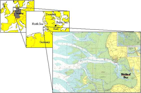
Figure 3: Area of investigation
Numerical model and in-situ measurements: The 2DH Flow Module of the Delft3D Modelling System was used to simulate water levels and current velocities. A curvilinear grid with 30,000 elements and grid spacing ranging between 60 and 180m was set-up initially. Details of the model development and calibration can be found in Palacio et al., 2000.
GUI for the investigation area: Figure 4 shows the GUI set-up for the study in question. Within the investigation area five gauge stations, operated by the relevant authorities, monitor the water levels continuously. Measurement campaigns of velocities using ship mounted and stationary ADCP are carried out at regular time intervals (every 3 months) and after relevant events as part of the research project Promorph. In Figure 4, all available transects are displayed and the data can be assessed by the user.
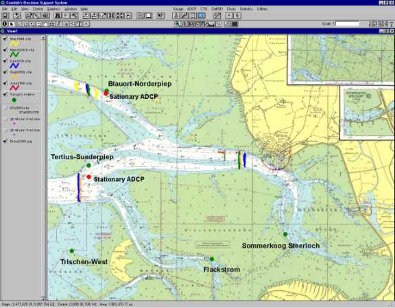
Figure 4: GUI indicating the location of the measurements
Database: The measurement data and model results files have been stored in the database set-up for the investigation area. To give an idea of the amount of measured data, during the Promorph project a four-day measuring campaign collects around 170MB. In addition, the model simulation (CPU time is about 100min per day of simulation on a 400MHz PC for a 30,000 cell model grid) creates result files that are usually of large size (around 110MB per day of simulation for the same 30,000 cell model grid and results every 15min).
Figure 5 shows a zoom of the investigation area with the location of some ADCP transects (in yellow) and the corresponding database tables that support these selected features. The database tables are used in conjunction with the GIS map layers in such a way that the database can be queried selecting objects in the maps thus increasing the flexibility of the graphical output. Data from the database are readily available and can be queried or used directly in any graph.
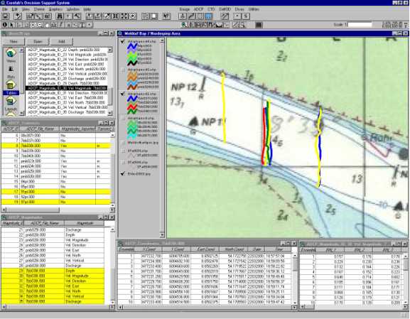
Figure 5: ADCP transects and corresponding database tables
Model calibration: The DSS has been used successfully in the calibration of the model. A significant number of model runs have been carried out with different model settings. The DSS speeds-up the comparisons between model results and measurement data. Figure 6 shows an example of the comparisons between measured and computed water levels carried out in the calibration of the model.
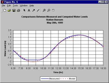
Figure 6: Measured versus computed water levels
Figures 7 and 8 show comparisons of measured and computed velocities along a transect respectively in terms of depth-integrated velocities (magnitude and direction) over the cross-section and in the form of vector fields. The statistical tools supported by the DSS enable the user to take decisions with respect to the optimum model settings.
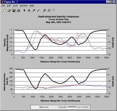
Figure 7: Measured versus computed depth integrated velocities over a transect for a given time
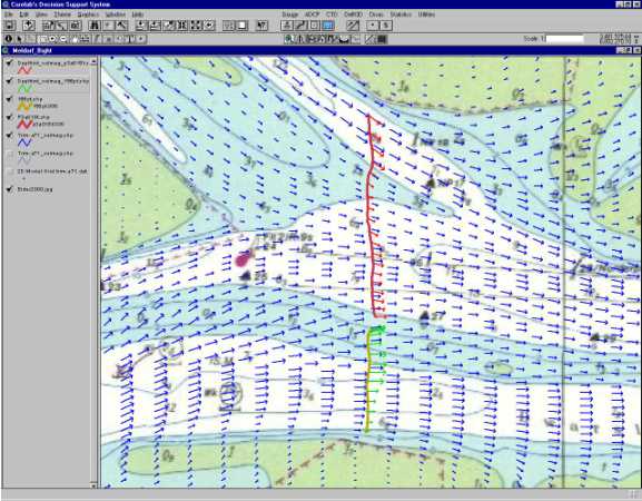
Figure 8: Measured versus computed velocity vectors for a given time
Output into reports: For the cross-section in question, 36 transects covering a tidal cycle were gathered. For every model setting, comparisons between model results and measurement data as well as their discrepancies need to be prepared. The DSS enables such set of plots to be prepared in batch mode and to output them directly to reports on pre-formatted sheets. The statistical analysis obtained with the resulting discrepancies (differences between model results and measurement data) obtained from the various runs are stored and help the modeler to select the most adequate model settings.
4. Conclusions and Future Developments
The use of GIS technology in the model calibration and validation brings many new capabilities and commodities to the model developer. This paper shows the applications of this technology to develop a DSS that assists the modeler in integrating measured data and model results for model development. The DSS has been tested successfully with a real world problem with huge amount of data. Alternative extensions can be coupled with this DSS for assisting the modeler mapping, preparing and handling input model data.
Acknowledgments
The authors would like to thank the German Ministry of Education and Research for funding the project and the Office for Rural Development (ALR) in Husum for providing the measurement data. Our gratitude goes also to Mr. Jan Schoppenhorst for his contribution in the development of the DSS.
References
Environmental Systems Research Institute, Inc., Esri (1996b), Avenue, Esri, Redlands, California.
Environmental Systems Research Institute, Inc., Esri (1996a), Using Arc View GIS, Esri, Redlands, California.
Palacio, C., Winter, C., Mayerle, R., COASTAL RESEARCH LABORATORY, 2000. Meldorf Bight Flow Model. Model calibration using the May 1999 field data. Report nr. 04-00, November 2000.
Rahtlev, Jürgen, CVGK and GK software user manual. Institut fuer Angewandte Physik, 1998.
RD Instruments (1994), ADCP User's Manual, RD Instruments, San Diego, California.
WL Delft Hydraulics (1999), Delft3D-FLOW, WL Delft Hydraulics, Delft.
WL Delft Hydraulics (1997), Viewer Selector, WL Delft Hydraulics, Delft.
Zielke, W., Mayerle, R., Groß, G. Epprl, D.P. and Witte, G., Prognose mittelfristiger Küstenmorphologieänderungen PROMORPH, Unterlagen zum Antrag, March 1998.
Fernando Toro, M.Sc.
PhD student,
Coastal Research Laboratory, Institute of Geosciences, University of Kiel,
Otto Hahn Platz 3, 24118 Kiel,
Germany;
Phone: +49 (431) 880 2548; Fax + 49 (431) 880 7303;
Email: ftoro@corelab.uni-kiel.de
Roberto Mayerle, Prof. Dr.
Director,
Coastal Research Laboratory, Institute of Geosciences, University of Kiel,
Otto Hahn Platz 3, 24118 Kiel,
Germany;
Phone: +49 (431) 880 3641; Fax + 49 (431) 880 7303;
Email: