LIDAR (LIght Detection And Ranging) has been a valuable survey tool since the early 1970s; however, only recently has enabling technology advanced to outfit a production aircraft with a high-performance, affordable system. This paper describes the general theory and operation of modern, robust LIDAR systems followed by project examples illustrating the value of remote-sensed LIDAR data for analyzing and predicting NW forest timber stand characteristics providing the basis for inventory evaluation.
The development of airborne laser scanning began in the 1970s with the first US government- supported systems. Although these systems were cumbersome, expensive, and limited to specific applications (such as, simply measuring the accurate height of an aircraft over the earth's surface with a single pulse), they demonstrated the value of this remote sensing/surveying technology. By emitting a laser pulse and precisely measuring the return time to the source, the "range" can be accurately calculated using the value for the speed of light (similar to a total station laser-surveying instrument), and be accomplished very rapidly.
The advent of GPS measuring systems in the late-1980s provided the necessary positioning accuracy required for high performance LIDAR. Within a few years, rapid pulsing laser scanners were developed, linked to the GPS system. The systems became complete with ultra-accurate clocks (for timing the returns or echoes) and Inertial Measurement Units (IMU) for capturing the orientation parameters or attitude (tip, tilt, and roll angles) of the sensor.
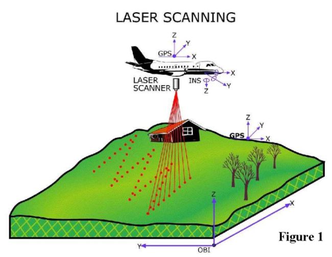
A LIDAR system is an aircraft-mounted laser system designed to measure the 3D coordinates of features from reflection (or echo) on the earth's surface. The most common laser wavelength used in topographic systems is near-infrared (1064 nano-meters) which is eye-safe, and provides an excellent return signal from vegetation and the bare earth.
The most advanced systems have wide operational capabilities and can establish a digital elevation model (DEM) with a point spacing from 1 to 15 meters with vertical accuracy of RMSE-15 centimeters. Figure 1 is a graphic representation of LIDAR data collection.
The raw LIDAR data must be processed to yield meaningful results. The GPS positions and the IMU orientation data are used to compute the position of the laser spot on the ground. Since the system has been calibrated, the accuracy can be validated with very little ground truth or survey points. Following this initial stage of processing, the points are then classified and surface features, such as, vegetation and buildings, can be separated, analyzed or removed to yield a bare earth model. Figure 2 is a TIN (Triangulated Irregular Network) of a forest site before feature removal; Figure 3 is a TIN the same site following feature removal; the area shown is 2000 meters x 3000 meters.
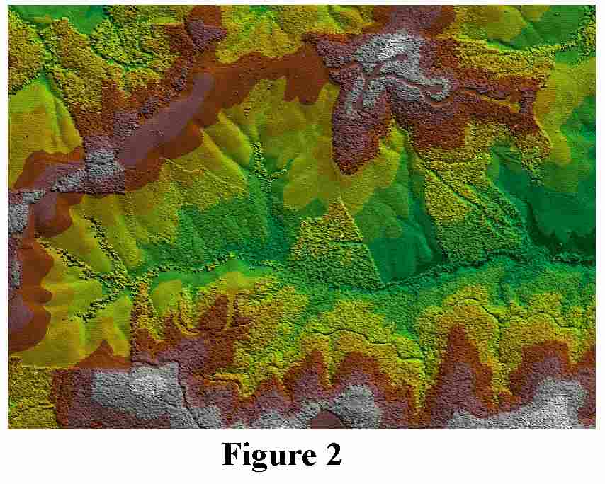
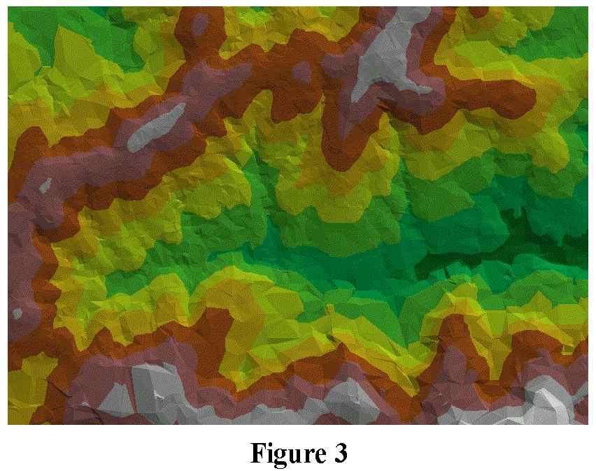
Note that Figure 2 is similar to an aerial photo image, and features (vegetation patterns, clear-cuts, drainages, and riparian vegetation) can be identified, and additionally, the data is 3D. Through surface analysis, the data has been classified, and points determined not be 'on-the-ground' have been removed to create Figure 3.
Since LIDAR is an active system, data may be collected during "clear" weather conditions, day or night. This flexibility is useful for many applications requiring data capture in areas prone to daytime fog.
On clear-hit surfaces (roads, parking lots, building tops), LIDAR points are typically within 15-cm RMSE vertical accuracy; on soft surfaces and vegetation, the vertical accuracy is dependent on the vegetation density; thus, variable. LIDAR systems capable of capturing multiple return values per discrete pulse can produce 'last returns' which are on or near the ground. In areas with vegetation cover, the vertical accuracy is a direct function defined by the density of the cover types and the density of LIDAR points 'hitting the ground'. Project design based on the complexity of the ground cover and terrain extremities will compensate for most design issues which will result in digital terrain models suitable to support 'forest management' 6-meter contours, as a minimum. It is not unusual for LIDAR-forestry DEMs support 3-meter or even 1.5-meter contours.
LIDAR is a very consistent sampling methodology as the collection process depends on precision engineering and machining principles; repeated analysis indicates that the standard deviation of calibrated systems is typically within 3 - 7 cm. The resulting data sets captured in a forest cover setting are ideal for analysis utilizing statistical analysis procedures proven by professional forests and land managers.
As with all remote-sensing applications, LIDAR is capable of acquiring vast amounts of accurate data without direct contact with the subject. For forestry applications, this measuring technology is extremely useful to minimize field time and personnel safety issues; data may be collected day, night, or in shadowed or hazardous areas. Characteristic applications include forest management planning, landslide or hazard assessment, surface runoff management, and data visualization. LIDAR-based data is typically more complete and usually more accurate compared to traditional methodologies. This paper builds upon these principals, and describes how LIDAR data sets may be utilized for prediction on forest biomass characteristics.
In 1999, a research project conducted on the HJ Andrews Research Forest in the Western Slopes of the Oregon Cascades resulted in strong relationships between small-footprint LIDAR data for prediction of stand height, stand basal area, and stand volume. The solid evidence from this study proving the validity of a LIDAR approach in a 'research environment' led to application of the same relationships and analysis for a 'commercially managed' forest.
Currently, industrial forestland managers inventory 10 - 15% of a typical tree farm each year, so a complete inventory requires 5 to 7 years. Often the inventory plot data is collected with variable reliability, and discrepancies between projected yields and harvested volume may differ by as much as 20%. Field collection procedures yield one data set describing the forest; LIDAR by comparison yields several data sets as previously described.
Having a LIDAR data base collected within a few days and calculating key inventory predicted characteristics are of immediate value, and can provide an excellent base for long-term forest growth models.
The LIDAR data for the industrial forest sites was collected with an AeroScan LIDAR, small-footprint system in October 1999 with 3.5-meter nominal post spacing. Note that 3.5- meter post spacing appears to be an efficient and cost-effective collection frequency, particularly when compared to traditional mapping techniques.
Ground data (inventory plot information) was provided by the landowner consisting of field inventory plot data for 31 stands which were chosen to span the full range of heights and stocking levels present from a larger list believed to be representative of the entire tree farm. Stocking was indexed by Stand Density Index (SDI) to provide more useful equations. The available data included average stand height, basal area, and volume; measurements for these stands were completed to coincide with the LIDAR data collection as close as possible: 1998 and 1999.
Although LIDAR data was collected for all 31 stands and processing/analysis was performed, this paper is using one of four areas to illustrate the study. This site was chosen because it represents a good sampling of the stand characteristics and terrain variability.
Graphics and various GIS applications were performed in ArcView 3.2 and ArcInfo. Statically analysis and regression fitting of data sets was performed in SAS software to explore relationships between LIDAR data and ground plot measurements.
Raster images with 10-meter and 15-meter cells were produced showing vegetation top (surface elevation models) based on the 'first-return' data set. Figure 4 is a TIN of the study site canopy layer produced in ArcView - 3D Analyst:
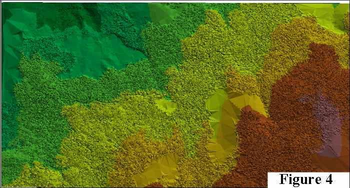
Figure 5 is the same area as a 'bare earth' TIN with the vegetation removed. This process began with the 'last-return' LIDAR points, or those points most likely to be on or near the ground. Surface analysis and aboveground point removal was conducted for development of this surface.
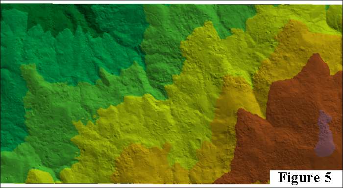
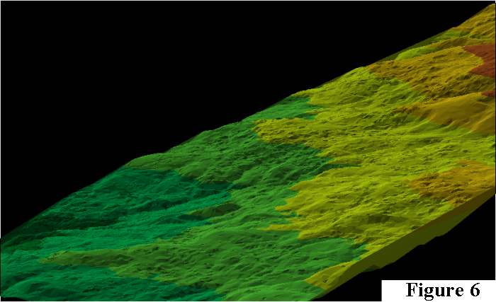
Figure 6 is a 3D view of the study area illustrating the terrain complexity of the area.
Vegetation top (that is, near the canopy) elevation was calculated as the highest first return in the cell; estimated ground elevation was calculated as the lowest last return in each cell. Vegetation height in each cell was calculated by the difference of these two values.
Figure 7 is a raster image displaying canopy height with the management unit boundaries; note the discrepancies of unit boundary polygons:
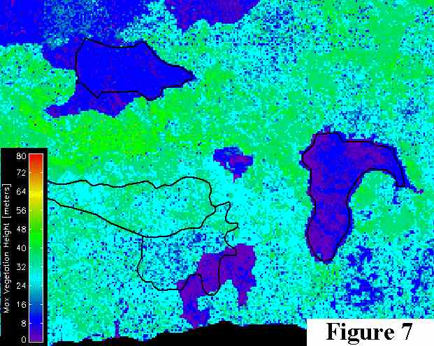
The stand boundary polygons provided did not often match the physical stand boundaries. This occurrence can be normal; as cutting boundaries are usually not required to follow stand boundaries. The stand boundaries for this study were adjusted in ArcView to follow physical stand boundaries as indicated by vegetation height.
These stand boundaries were then buffered in ArcView to avoid edge conflicts and the resulting polygons were exported to the SBG LIDAR Analysis routines. This step created ASCII x-y-z files for use in SAS software for regression analysis.
Based on the LIDAR pulse density, about 100 pulses appeared to be adequate for calculating percentiles of height and cover in a cell of 20-meters, which was logically chosen for this analysis. For each cell, height percentiles and cover percentiles ranging from 0% to 100%-ile were calculated. Average height and cover percentiles were calculated for each stand; maximum height for each plot was also determined. These LIDAR measures were used to build models for statistical analysis.
The final step was to explore the relationships between ground data and LIDAR measures using stepwise (therefore several variable equations) in SAS. Predictor variables derived from the data were average maximum height, average mean height, height percentiles, and canopy cover percentiles. From rigorous analysis and testing, good fits were obtained for each stand characteristic using the plot data provided.
The following figures illustrate these relationships by theme:
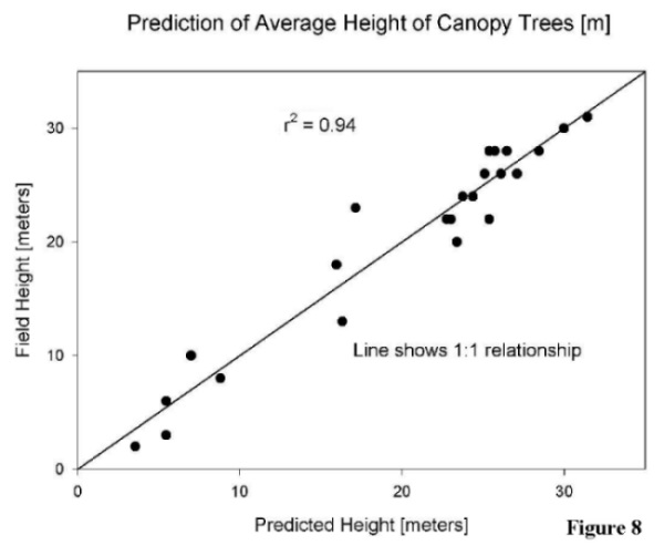
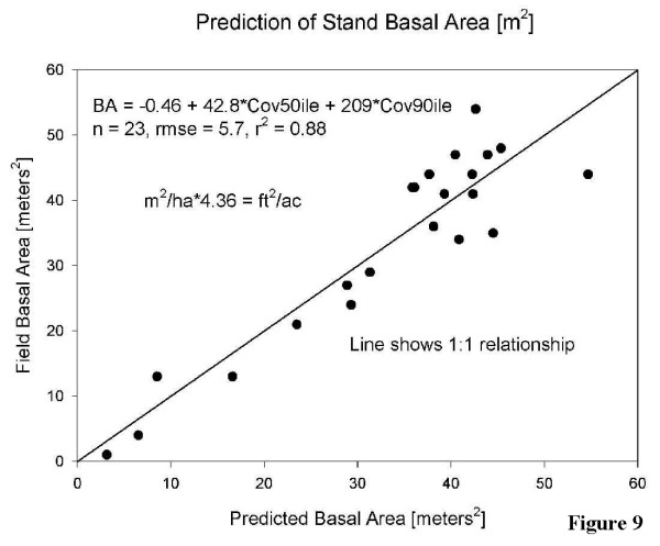
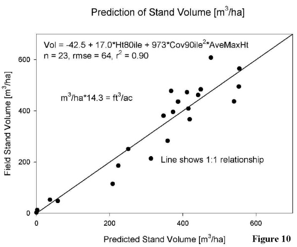
The results are quite good and measure up very well to traditional inventory techniques.
LIDAR technology has come-of-age to service the requirements of the forestry land management community. The processing of the data for meaningful applications is proven, and the user community should consider LIDAR as another 'tool in the toolbox' for mapping, evaluation, study, and analysis of forestry biomass.
The user community should be conscious of absolute accuracy, and apply the data with full recognition of the collection procedure and product development. Applied correctly, LIDAR is a very useful database for most forestland applications.
"LIDAR Industry Status" - Michael Renslow, First International LIDAR Mapping Forum, Denver, CO, Feb. 8, 2001 (www.lidarmap.org).
"LIDAR: The Equipment and Technology" Michael Renslow; Land Surveyors of Washington 2000 Annual Conference Proceedings; Feb. 17, 2000.
"Operational Visualization Applications Using LIDAR Data" Hill, Gloyna, Chavez, Young, EOM - November 2000 Issue.