Figure 1.� A GIS model representation of a wetland
Geographic Information System (GIS) objects such as points, lines, polygons, and grids are often used to represent and model physical features that are displayed on maps.� By overlaying and intersecting these objects, values are selected and quantified to represent the interactions of these objects.� Often, GIS objects are represented as having static values for modeling; however, the physical features that they represent may vary.� This paper examines a method of quantifying the variability found in physical features when performing GIS modeling.� Two hypothetical examples illustrating this method are also provided.
A standard method of applying GIS modeling is to identify the physical features to be modeled and then represent them with different GIS shapes and themes.� The values of these features are stored in the attributes of their representing shapes.� Polygons are often used to represent physical features with areas.� Creating a grid from a set of feature points provides a means of converting point information into area information.
The interaction of these shapes by overlaying one on top of another may provide useful information.� The resulting intersections between shapes may be used to calculate information using their related attributes.� For example, a polygon representing a forest may be overlain with another polygon representing a burned area from a forest fire.� The intersection between the two can be used to quantify the amount of timber destroyed by the fire.
Converting point data into a grid provides a spatial means of representing an area that is not completely filled with points.� Grids are very useful in displaying spatial trends in data and provide a smooth and consistent method of applying point values across an area.� Values from the grid nodes can be selected and manipulated for calculation purposes.
A grid that has been created from a set of points may be intersected by a polygon.� This intersection can then be used to select grid points.� Once selected, a calculation can be performed on them.� The resulting value can then be assigned to the polygon.� Conversely, the intersecting polygon�s value may be applied to each of the grid nodes within the intersection.
For example, a set of points representing metals concentrations in soil can be gridded to represent the area concentration for a site.� A proposed remediation for the site is to excavate all soil down to a depth of 1 foot and dispose of it into a solid waste landfill.� The cost of removal is related to the metals concentration of the soil being landfilled.� The excavation boundary can be overlain onto the grid, and an estimate of the concentration of the soil being removed can be calculated.
In the soil removal and forest fire examples, an assumption was made that the polygon and grid shapes do not vary; however, they often do.� The delineation of the polygons or the process that the polygon represents may be imprecise.� In the forest fire example, the polygon representing the burned area may have been digitized from air photos.� From these photos, truly delineating the boundary with a high degree of accuracy may be difficult.� In the soil removal example, the excavator may only be able to approximately follow the removal boundary.� So no matter how sharp and accurate the modeling shapes appear on a map, the situation in the field that they represent is almost always much less clear.
At least three general types of uncertainty may influence the modeling shapes:
Uncertainty in measurements can be caused by inaccurate digitizing or by delineating an area with an imprecise device.� For example, a wetland may be delineated using a geographic positioning system with poor precision.
Changing physical characteristics are often observed in nature.� Vegetation growth and an evaporating pond are two examples of physical characteristics that might be represented with a polygon but would undergo a change in their true boundaries over time.
Subjective interpretation of areas on maps is another source of variability.� Two individuals given the same data will often draw slightly different boundaries with the data; therefore, a boundary drawn on a map using �best professional judgment� is implicitly fuzzy.
This paper explores the use of the Monte Carlo and bootstrapping methods to quantify uncertainty.� The Monte Carlo method is essentially the process of placing a model�s variables into an algorithmic loop and allowing them to change based on certain conditions.� Often these conditions are chosen at random from known distributions.� Each time the variables go through the loop (i.e., one realization), the results vary according to the probabilities of the condition�s parameter value. .� The results are stored, and a list of variable outcomes is constructed.� Bootstrapping is an algorithmic device that allows the creation of nonparametric distributions.� It does so by taking a set of data, choosing members from the data set for replacement, and building a new data set.� Both methods can be implemented straightforwardly.
Shapes such as polygons or grids are manipulated so that they can change shapes and values.� These changes take place within the Monte Carlo algorithm.� For each realization, random values from distributions are selected and cause the size of a polygon or the values of a grid to change.� The interaction of the variable shapes with the other GIS components of the model allows variable results to be recorded and a final list of results to be constructed.
The method for incorporating uncertainty presented in this paper focuses on changing polygon size and grid values within the Monte Carlo algorithm.� Using a size parameter, a polygon can be expanded or contracted.� The change in polygon size for each time step models a physical feature that is known to vary.� The size factor is chosen either at random or from a distribution.� A new grid is created for each realization by adjusting the point values before the grid is created.� Point values may be altered using known distributions or by bootstrapping.� The resulting grids are used to represent the variability inherent in the point values.
The general algorithm for the method is as follows:
� First, a model is created by representing variable features with polygons and a set of points
� Next, a Monte Carlo algorithm is added with each pass through the algorithm representing a single realization of the model
� Each point value in the data set is adjusted using a distribution or bootstrapping
� The newly adjusted point set is used to create a grid
� A size parameter is chosen either at random or using a distribution
� The polygon is expanded or contracted based on the size parameter
� The polygon intersects the grid and selects grid values
� Calculations are performed on the selected grid points
� The results are stored and the algorithm continues to the next realization
� Once the total number of realizations in the simulation is reached, the model stops
� The stored results are used for analysis.
The changing of the polygon shape and grid values from one realization to the next is used to quantify variability in the features that the GIS objects represent.
The following two hypothetical examples are used to illustrate the method of incorporating variability into GIS shapes.� The first example describes the modeling of a wetland and the interaction of a bird with a pesticide.� The second example describes the economic interaction of a forest with an endangered species boundary.
A wetland example
Assume that a field is often partly covered by shallow water.� The area of the water will vary throughout the year owing to rainfall, evaporation, and drainage.� Water birds find the shallow water of the field a perfect habitat for feeding.� The birds do not feed on any of the field�s dry portions.� The bird population does not migrate and lives year-long in the vicinity of the field.�
The field has been under agricultural use for many years, and, consequently, pesticide residue has built up in the soil.� During the past few years, more and more of the birds in the vicinity of the field have been dying.� The pesticide is suspected as one major factor in most of the deaths.�
As part of an ecological study, a value for pesticide exposure is being determined by taking the average concentration of the pesticide within the bird�s feeding habitat (i.e., the flooded portion of the field) and dividing this average concentration by the size of the feeding habitat.
During the study, several phases of soil sampling have been conducted to characterize the pesticide distribution in the field�s soil.� These sampling locations are scattered throughout the field somewhat randomly.� This sampling shows that the distribution of pesticide is generally heterogeneous.� A series of air photos has also been used to investigate the changes in the flooded portion of the field over time.� These changes in area appear to roughly follow a normal distribution.
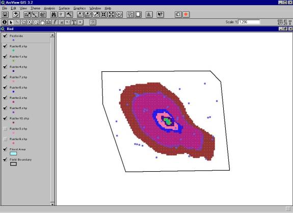
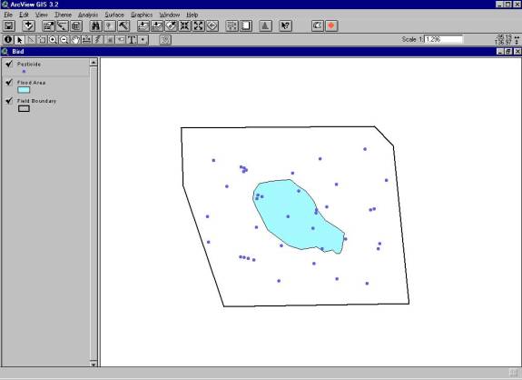
A GIS model (Figure 1) is assembled to quantify the bird�s exposure to pesticide in the feeding habitat.� In a nonvarying system, the average size of the flooded area would be determined from the area photos and overlain onto the field.� A pesticide concentration grid would then be created and placed onto the field.� The intersection of the flooded area would then be used to select grid points within the intersection, and an average of these points would be calculated.� The average pesticide concentration would then be divided by the area of the flooded portion of the field.
|
|
|
Figure 1.� A GIS model representation of a wetland |
However, because of the varying flooded area and the heterogeneous distribution of the pesticide soil samples, we wanted the exposure values to be expressed as confidence intervals instead of as a single set of values.� To do this, the model was altered in the following manner.
A Monte Carlo loop was created.� The polygon representing the varying flooded area within the field was allowed to change its size based on values chosen from a normal distribution.� This distribution was assumed from empirical data acquired by observations of the flooded area�s shape.�
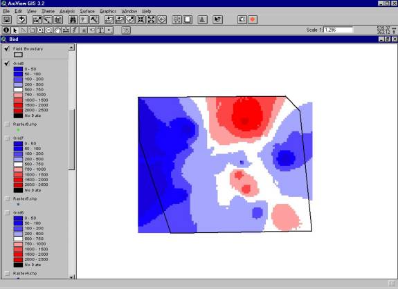
The soil sampling points were bootstrapped during each realization, and a new grid was created from these data sets.� Bootstrapping the sampling points is used to quantify the heterogeneity within the set.� Because samples with high pesticide concentration are in close proximity to samples with low pesticide concentrations, a slight change in sampling location may have a large impact on the total pesticide grid.� Bootstrapping the pesticide samples simulates re-sampling the field in different locations and provides a means of calculating the variability in the pesticide samples.
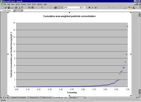
The polygon for one realization then intersected the grid for that same realization, and an average pesticide value and flooded area value were obtained and associated.� A distribution of these associated values was built, and the confidence values were found using the percentiles.� The results of this analysis are displayed in Figure 2.
|
|
|
Figure 2.� Distribution of area-weighted pesticide concentration |
The median area-weighted pesticide concentration value is 0.065 (μg/kg/ft2).� The 5th percentile value is 0.007 μg/kg/ft2, and the 95th percentile value is 4.4 μg/kg/ft2.� These values are applied to further exposure calculations providing a quantification of the variability in the two exposure components.
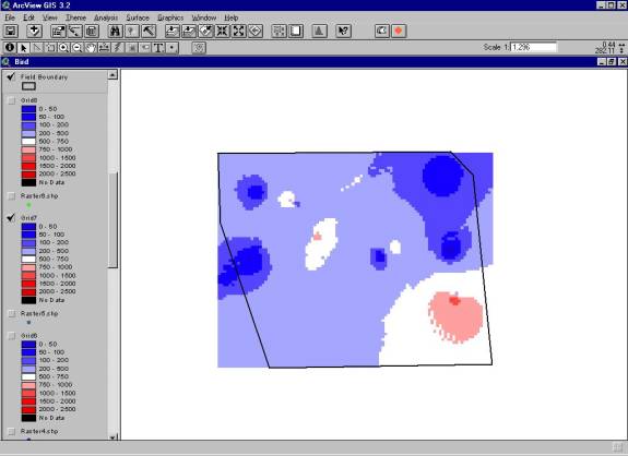
In this example, the changing of the polygon was used to represent the growing and shrinking of the flooded area from physical phenomena (Figure 3).� The bootstrapping of the pesticide samples is used to evaluate the heterogeneity of the samples.� Because bootstrapping chooses and excludes samples in the data set that are being gridded during each realization, mainly samples with higher values can be chosen one time, and mainly samples with lower values can be chosen the next time (Figures 4 and 5).� This method is used to represent sampling of the same area in different locations.
|
|
|
Figure 3.� Example of varying polygons for each realization |
|
|
|
Figure 4.� Pesticide grid created from a bootstrapped sample set for one realization |
|
|
|
Figure 5.� Pesticide grid created for a different realization (note the differences in concentration) |
The second example involves a parcel of forestland that is available for a timber sale.� Crews have gone out into the parcel and collected tree cores from representative parts of the forest.� These cores are used to estimate the amount of board feet available for the timber sale.� The board feet estimates provided by the cores are known to vary normally.� The cores were collected from a relatively uniform grid.�
An endangered species is known to inhabit a portion of the forest near the timber parcel, and past field investigations have found that the species range intersects a portion of the timber parcel.� Different investigations have delineated different boundaries for the endangered species.
The timber company owning the parcel would like to know the potential economic impact that the endangered species might have on their upcoming timber sale.� They would also like to incorporate the variability of the board feet estimates into the quantification so that they might have some degree of confidence of what the economic outcome of the sale might be before proceeding with the sale.
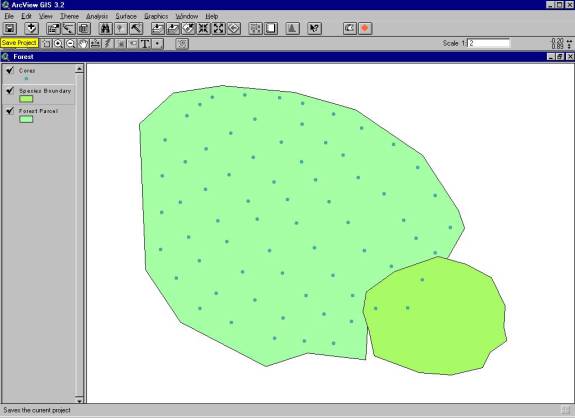
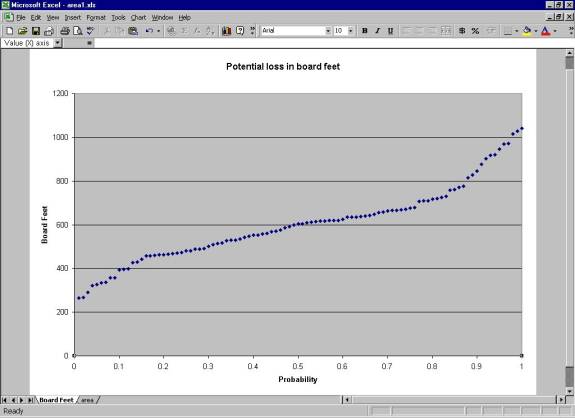
A GIS model (Figure 6) is assembled that represents the timber parcel as a polygon, the cores as points, and the endangered species boundary as a polygon.� A grid of board feet is made from the core samples.� The grid values for the timber parcel are then summed to calculate the total potential board feet available for the sale.� An average endangered species boundary intersects the grid.� The board feet grid values are selected within this boundary and the amount of board feet potentially lost is determined.� Figure 7 displays the distribution of board feet loss.
|
|
|
Figure 6.� The GIS model of the forest example |
As in the previous example, a Monte Carlo algorithm was created, and the species boundary and board feet grid were allowed to vary.� For each realization, a new value was selected from a normal distribution.� This distribution was assumed based on past experience and field observations.� .� The size of the endangered species boundary was selected at random from a uniform distribution.� The maximum and minimum sizes observed in the field were used to define the extremes of the distribution.� The resulting board feet lost were recorded for each realization, and a distribution of loss was generated.
|
|
|
Figure 7.� Distribution of board feet loss |
Figure 7 displays a median value of 605 board feet lost from the impact of the endangered species boundary.� The 5th percentile value is 325 board feet lost, and the 95th percentile value is 946 board feet lost.
�
This paper has presented a method that may be used to quantify some types of uncertainty found in GIS modeling.� The main aspects of this method rely on modifying a model so that it may be operated using a Monte Carlo algorithm.� The size and shape of polygons and the values of grid GIS objects are allowed to vary based on known distributions or by bootstrapping.
The resulting distribution of results can then be used in regulatory and economic analysis.� The estimate of variability that this method provides can be used as an important tool for the interpretation of modeling results.