This paper describes an application built by the NAFTA Intermodal Transportation Institute at Dowling College. The NAFTA Institute develops applications and analyzes transportation impacts of trade between the North American Free Trade Agreement (NAFTA) countries of Canada, Mexico, and the United States. This paper discusses the development of this Trade View application together with design issues and trade-off analysis. The final application design is presented including the MS Access database, VBA, and SQL application code and ArcView Avenue scripts. The paper describes how GIS can be combined with other data processing systems to build integrated applications.
The NAFTA Intermodal Transportation Institute at Dowling College is funded under a grant from the United States Department of Transportation (Federal Highway Administration). The grant is managed and administered through the Department of Transportation of New York State.
The Institute focuses on providing transportation information and developing solutions to transportation issues resulting from the impact of North American Free Trade Agreement (NAFTA) related trade issues. We also provide support for small and medium size businesses that want to start or increase exports and/or imports to/from the NAFTA countries of Canada, Mexico, and the U.S. In support of these two missions we operate a web site at www.naftainstitute.org
The NAFTA Institute is operated through a partnership between Dowling College and the University of Texas at El Paso (UTEP). We serve several types of users including transportation planners at all levels of government; national, regional, and local. We also serve planners and managers in the transportation and trade industries. In addition we provide resources to small and medium sized business managers.
The Institute is directed by a combination of internal and external management. Our steering committee is made up of administrators and faculty from the two colleges. Our advisory council is made up of government and industry stakeholders. These are government officials and business people from entities that have a large stake in more efficient trade between the NAFTA countries. The members of the advisory council are from agencies and companies external to both colleges and the New York State DOT. The steering committee and the advisory group work together with the management team from the NYS DOT to direct and manage the operations of the Institute.
Many of the planners in the state Departments of Transportation (DOT) and others have complained that there is not enough timely information on trade corridors that are resulting from NAFTA Trade. The traditional approach to developing this data is to have researchers gather data, manipulate it using relational database management software and GIS systems, than publish or present the data at appropriate conferences. An example of this approach to corridor mapping is shown in figure 1 below. This paper, based on the work of McCray and Harrison (University of Texas) was published in January 1999 and currently serves as the de-facto NAFTA corridor definition. The basic problem is that the data, published in 1999 is based on 1996 trade data. Therefore, the corridors presented are what existed in 1996. Although useful for understanding historical and representative trade flows, not timely enough for most planners.
Another problem with the traditional approach to corridor maps is that specialized skills are required to develop these maps. That is why researchers can only periodically publish these reports.
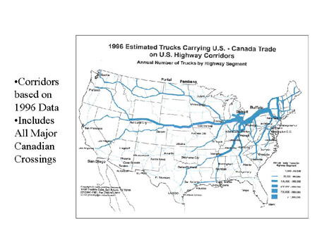
The information that the transportation planners are looking for is shown in figure 2 below. The corridor map shows the main highways used by NAFTA trade carrying trucks. The routes carrying the most trade or largest number of trucks are drawn with the thicker road symbols. This provides an easy way to see the routes that are most impacted by NAFTA Trade. However, a limitation to these traditional corridor maps is that they are typically developed for the full national flow of trade from all the major border crossings. If a DOT is interested only in the traffic crossing at a single border crossing or even all the crossings in a single state, this information is not available from the traditional reports.
Our stakeholders asked the NAFTA Institute to develop an application that would allow non-technical and non-GIS personnel to produce these corridor maps in a more timely fashion. They wanted the application to be easy to use and require no specific technical skills. The application should run on a standard PC platform so it can be made available to the widest audience. The application should use well known and understood public or readily available data sources. The application also needs to balance performance and utility so it will be as useful as possible but still perform acceptably on a standard PC.
The approach we took for this project was designed to allow the NAFTA Institute to develop the required skills, design techniques, and software routines to accomplish trade corridor development. We planned to perform this development at the NAFTA Institute using student interns and workstudies.
We also wanted to build the application in a manner such that new trade data and road networks could be introduced without complete redevelopment of the application. This will allow for future enhancements as new data becomes available.
Our approach included a multi-staged development plan that would create incremental versions of software. The initial version would become version 1.0. We hoped to establish design issues with version 1.0 so that we could address improvements to design limitations in later versions of the software. User feedback and knowledge gained from the use of version 1.0 would be used to make continuous improvements to the software at later releases of the application.
In order to allow the distribution of the application to a wide audience without requiring expensive data license fees, we decided to build the trade database for the NAFTA Trade View Application using the U.S. Department of Transportation, Bureau of Transportation Statistics (BTS-DOT) Transborder Surface Freight Data. This is a free federal data source that is commonly used to study NAFTA Trade Flows. This data is available as monthly files at the BTS web site. This allows for easy and timely update of the trade view application data.
We also decided to use the readily available Office Productivity tool, Microsoft Access as the database for storing and manipulating the NAFTA Trade data. This is a powerful database application that most of our constituents have as part of their Microsoft Office installations. Using this database, we felt we could offer the application to the largest number of users.
After consulting our constituent users, we found that the prevalent GIS software that they had available was the widely distributed ArcView desktop GIS. Therefore, we decided to use ArcView as the GIS for trade corridor map development, display, and manipulation.
In order to have an application that would perform reasonably on a standard PC we decided to pre-establish trade routes in the transportation highway network. We would then join these routes with the user selected trade data at run-time. Then we would sum the trade data by road section and use this attribute to generate the graduated symbol highway corridor map. We then would create routes between all the major NAFTA border crossings and the major population center in each State/Province. We used the shortest path route selection to approximate the routes that a truck might use to travel from the border crossing to each state or province destination. In order to have the system perform by using a smaller road network and to approximate the long haul corridors, we used the interstate highway network layer that comes with the standard ArcView GIS distribution. We also used the national highway networks that come with ArcView for Mexico and Canada. I believe these networks are derived from the Digital Chart of the World data.
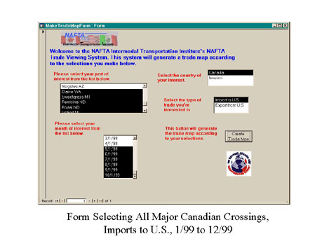
Our concept was to have an application where a user could fill out a simple form representing the corridor information that the user is interested in. Such a form is shown in figure 3 below. On this form the user would select the border crossings that they are interested in, the time frame they are interested in (by selecting a set of individual months), whether they are interested in imports or exports, and whether they are interested in Mexican or Canadian trade. The user would then click on a button and the application would automatically generate the corresponding corridor map. This user query form was developed in Microsoft Access.
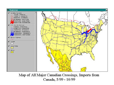
Once the information is filled in by the user, the query is processed in MS-Access to generate the trade data requested. The requested data is then processed to match the trade data and GIS route data for route/segment allocation and accumulation. Once the trade data per highway segment information for the requested query is generated, ArcView GIS is activated to display the final trade corridor map. An example of such a trade corridor map is shown in figure 4 below.
The BTS Transborder Surface Freight Database is published monthly and posted on the BTS Web Site. It typically takes a few months to publish the data, so the data on the web site lags the calendar month. The data is published as separate files for Imports and Exports and as separate files for Canada and Mexico. Therefore, there are four files all together for full monthly NAFTA trade flows. The trade data is published as Dbase Files. We import the Dbase files and append the file data to an MS-Access Database Table for Canadian/Mexico Imports/Exports. The BTS data provides a record for each combination of trade path, for a given month. For example, there is a record in the 1/2001 file for every path from any given Canadian Province (i.e. Ontario), through a particular border crossing (i.e. Buffalo as given by the DEPE Code 0901), to a particular U.S. State (i.e. Virginia). Therefore, for each record there is a U.S. State column, a Canadian Province or Mexican State column, a column for the DEPE code which indicates the border crossing the trade passed through, a column for the value of the trade over this path for this month, and a column indicating the month for this trade flow. This data layout is shown in figure 5 below.
By concatenating the DEPE code for the border crossing and the State code for the U.S. State, we can determine a trade value traveling over the path from a particular border crossing to a particular state. We can also perform a similar function by combining the Mexican State or Canadian Province and DEPE code. Of course the trade value is the same for both sides of the path since the same amount of goods must travel to the border crossing and from the crossing to the destination. This gives a trade corridor value for a single path on the highway network.
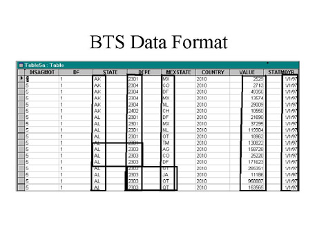
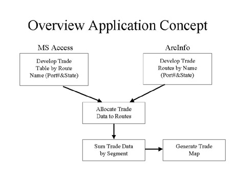
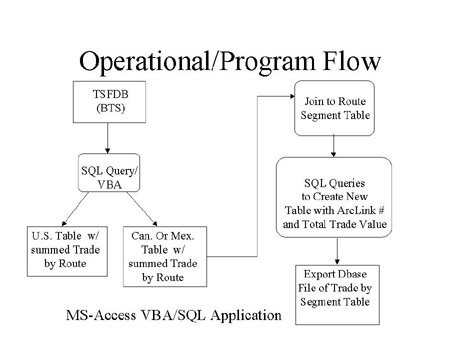
Figure 6 below shows the overall concept of how the NAFTA Trade View Application is designed to work. In MSAccess, a query, using the selections made by the user in the selection form, is executed to develop a table of trade amounts for each combination of port (border crossings) and destination states. These trade amounts are then matched against pre-determine network routes that have been labeled with the concatenated DEPE/State Code. For example, trade between Buffalo and Virginia will be labeled 0901VA. The network route between Buffalo and Virginia will also be labeled 0901VA. In this way the trade data and the route data can be directly related and allocated. The application then allocates the trade data to all the various routes that represent all the crossings the user has selected. The trade data is then summed for all routes crossing each individual highway segment. For example, a single segment of Interstate Highway 80 might be part of several routes from eastern border crossings to western destination states. We find all the routes that pass over each segment and add up the total trade value and assign it to the highway segment. The application then joins this trade data value field to the highway GIS data layer, using the segment ID Code as the common field. The trade corridor map is then generated by ArcView using a graduated symbol for the highway segment proportional to the trade amount.
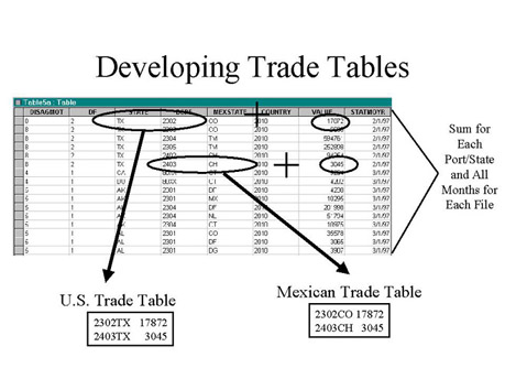
The first step in creating the trade corridor map is to generate the trade table by route in order to allocate the trade to the network paths. This is shown in figure 7 below. For any user query, either imports or exports, either Mexico or Canada, we need to query one of the four BTS trade tables. Since the table includes the trade data for a combination of source location, border crossing, and destination location, we actually generate two tables from the trade data, one for each country on the opposite sides of the trade flow (i.e. Canada and the U.S.). One table has a field that concatenates the DEPE code (border crossing port location) and the destination location codes. The other has a field for the concatenation of depe and source location code. Both tables have a field that represents the trade data amount. Therefore, each record in the original trade table generates a record in each of the resulting tables. For example, as shown below, the trade table generates two resulting trade tables, one for Mexico and the other for the U.S. The two records I have circled each result in an entry in each table. The first record generates an entry for DEPE 2302TX in the U.S. Table and an entry for 2302CO in the Mexican Table. Both of these entries have a value of 17872, since they represent the two halves of the trade flow; the U.S. side and the Mexican side. The second record generates a record for DEPE 2403TX in the U.S., and 2403CH in the Mexican table. Again the value is the same for both (3045) since they come from the same trade record.
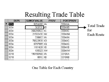
While we are breaking these trade records into their respective parts, we also sum the data for each combination of DEPE and source/destination codes for all the months the users has selected in the form. In this way we end up with both a U.S. and a Canadian or Mexican table that have the total trade for the whole time period asked for by the user. As shown below in figure 8 each of these two tables has a column for the DEPE (border crossing code), a column for the total trade value for trade traveling from the DEPE column crossing to the province (or state) in the next column, a column for the state or province or origin or destination, and finally, a column for the concatenated value of port (DEPE code) and province or state. This last column is of significant importance since this is how we can link the trade for this particular path to the GIS network path that the trade follows. The resulting table is shown in figure 8 below. The table now contains a record for each unique path from a particular port to a particular source or destination in the users query selection. Each record also contains the amount of trade traveling over that particular path.
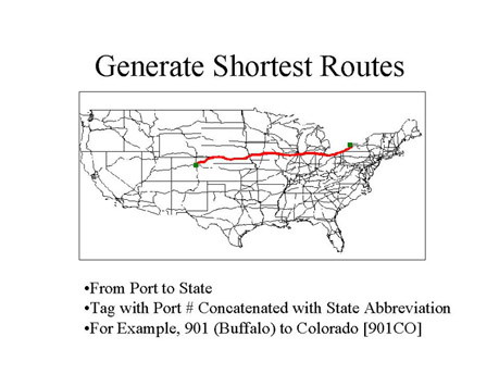
Now that we have a value for the total trade for each unique path resulting from the user's trade query we need to have the route to assign this trade value to. This is done through the use of ArcInfo's network analysis tools. Using the U.S. Interstate Highway layer as the base we select nodes at the major border crossings and nodes at major population centers in each destination state. We then have ArcInfo build a route from the port node to the state destination node using the shortest path method. In this way we approximate the route that a truck carrying international trade might travel from the port to the destination. Of course this route would likely be the same whether the truck is traveling from the state to the border crossing (export) or from the crossing to the state (import).
Once ArcInfo builds the shortest path route, we have it name that route with the concatenated value of the border crossing DEPE code and the two letter state abbreviation for the state the route goes to. This value of the route name becomes the value to link the trade amounts from the users trade query to the route for determining trade flow. The process of creating these routes is shown below in figure 9.
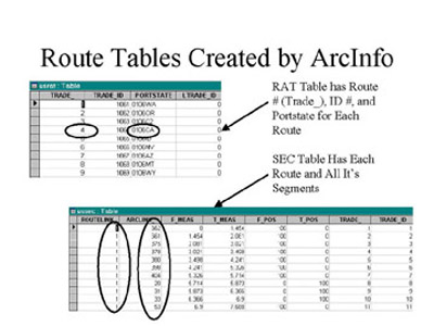
The method that ArcInfo uses in building these network routes versus the method that ArcView uses is critical to the functioning of the application. This key method is known as dynamic segmentation. When ArcView Network Analyst builds a route, it creates a new graphic feature that represents the path determined by the network analysis. When ArcInfo creates the route, it creates info tables that reference the graphic features in the network layer to indicate which network segments are part of which route. This capability is critical since we need to be able to identify many routes that might pass over the same highway segment. This would be very difficult in ArcView, but is a simple query to the tables created by ArcInfo. The tables that are created by ArcInfo are shown in figure 10 below. One is the route attribute table (RAT), the other is the section (SEC) table. In the case of the route system built for our trade view application the RAT table includes a unique route number for each route from a port to a state or province and the port/state or port/province label for the route. This last information is the key to linking the trade data to the route system for allocation.
The SEC table has a record for every segment of the network system that makes up each route that has been created. In our case, the key fields are the routelink field which identifies which route (by ID number) the segment belongs, and the Arclink field which is a pointer to the segment itself in the base highway network layer. These two tables allows the application to identify each route with all the segments that make it up as well as identify all routes that a given highway segment participates in. This is key to allowing for the allocation of trade as we will see later.
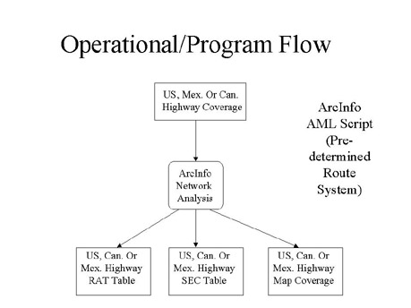
With these basics discussed, we can now describe how the application is actually constructed and how it operates. The program is modular to allow us to change parts with out re-writing the entire application. The first part of building the application is to develop the route network. This creates three separate files for each NAFTA country. In the Trade View Application these files are generated by an AML script. This script uses a file that contains the unique route IDs and the beginning and ending network nodes for each route. This file is maintained by hand. The script also uses a second file that contains the unique route IDs and the port/state or port/province label for each unique route. Again this file is maintained by hand. The AML script reads these files and runs the ArcInfo network analysis routines to create the shortest path routes between the designated nodes and adds an attribute field to the RAT for the port/state or port/prov label for each route.
Once the script is run, the result is a RAT table, a SEC table, and the Highway Network Map Coverage for each country, U.S., Mexico, and Canada. This AML script part of the Trade View Application is shown in figure 11 below.
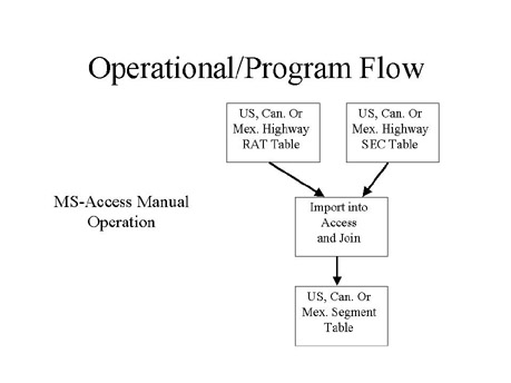
Once the various network tables are created for each country, these tables are then exported as Dbase files and imported into an MSAccess database. In the Access database, these tables are joined together so that each record contains the reference to the highway network segment, and the port/state or portprov label for the route the segment is in. In the resulting route/segment table a segment will appear potentially many times. Once for each route that it participates in. Each time it appears, it also identifies the port/state label for each route.
This import and join process as shown in figure 12 below, is a manual process that is performed once. The only time this process needs to be redone is if we use a new highway layer or change the method of determining the route paths. If we do make this type of change, as long as the result includes routes with the same port/state or port/prov labels, the new tables and map layer can be used in the rest of the application without further modifications. This is the modularity of the application design.
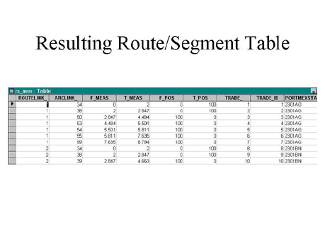
The result of the above process creates a route segment table for each NAFTA country as shown in figure 13 below. As can be seen, the joined table now contains a record for each segment of each route. The routelink field contains the route id for the unique network route path. The Arclink field includes the pointer to each segment in the highway network coverage that makes up the route. And, in this case, the portmexstate field contains the label for the route from the port (as indicated by the DEPE code) to the Mexican State (as indicated by the concatenated Mexican State abbreviation. (i.e. 2301AG). We are now ready to attach the trade data, sum it up by highway segment (Arclink Field), and produce a file for ArcView GIS to use to generate the Trade Corridor Map.
From here on out, the application can run automatically every time the user fills in the trade corridor request query form described previously in this paper. No more manual processes are required. There are two pieces to the run-time Trade View Application. The first part is shown below in figure 14. The second part will be described shortly.
The first part of the application is a piece of Structured Query Language (SQL) based Visual Basic for Applications (VBA) code that runs when the user clicks on the Create Trade Map Button on the Query Form. Based on the country of interest selected by the user, and whether imports or exports are selected, the application code queries the appropriate BTS Transborder Surface Freight Database table to select the data for the months and ports that the user has selected. This query produces a temporary table with the trade data summed for all the months selected for all of the ports (as selected by the user) and origin or destinations. One such file is created for the U.S. and one for the appropriate other NAFTA country. This new temporary table now contains a record for each unique combination of port (DEPE Code) and Source or Destination location (state or province abbreviation). Each of these records also contains the total trade for all the months selected for each network route path. Again, the key field here is the port/state field that identifies the route that the trade needs to be allocated to.
Once this temporary trade table is created, it is then joined to the existing route/segment table discussed above. This join is based on the common port/state or port/prov field. This join now results in the route segment table having the total trade for the user's query now appearing as a field for each segment record. We now run a second query on the resulting joined route/segment table to sum up the total trade for each segment by adding the value from all the records for routes that each segment appears in. The result of this query is now a new temporary table that contains only a record for each segment that has trade allocated to it. Each of these records contain the segment identification (Arclink field) and the total trade flowing over the segment.
Once these temporary trade by segment tables (one for each country selected by the user) are created the VBA application exports these tables as temporary Dbase files to a pre-defined directory that ArcView can access. The VBA code then unjoins all tables, deletes any tables no longer required, and sends a message via the DDE feature of windows to Arcview to execute the second part of the application. ArcView is also set to be the top active window so ArcView becomes active to display the resulting trade corridor map.
Once ArcView is active, an Avenue script (as shown in figure 15 below) is started that imports the temporary trade tables (one for each country) into the ArcView project. These tables are then automatically joined to the GIS Highway Network Shape files using the common Arclink field. At this point, the shape files now have a field containing the amount of trade flowing over each highway segment. The avenue script then executes commands to redraw the highway shape files with a graduated symbol and a pre-determined legend and symbology. This produces the final corridor map as requested by the user. The application and the map are now complete.
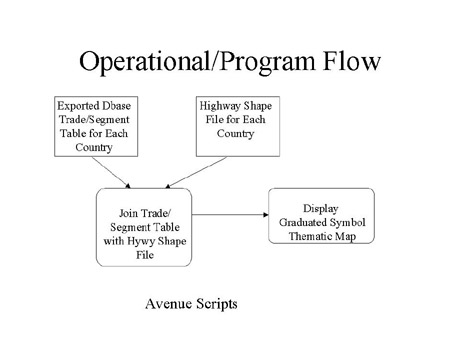
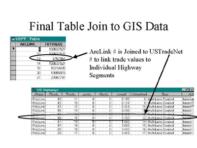
Figure 16 below shows how the trade data exported as a Dbase file from MSAccess is joined to the highway GIS layer in ArcView. The trade data file contains the Arclink field which links to the segments in the highway layer. For example, in this instance, the Arclink field joins to the USTradeNet field to link the trade data to the highway segments. A similar process is performed for the Canadian or the Mexican highway layers.
The result of all this data processing work is indicated in figure 17 below. We now have a GIS layer (a Shapefile) that has a field that contains the total trade flowing over each individual highway segment.
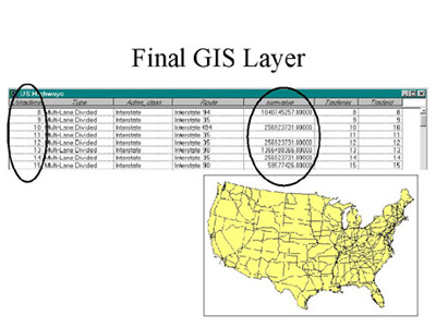
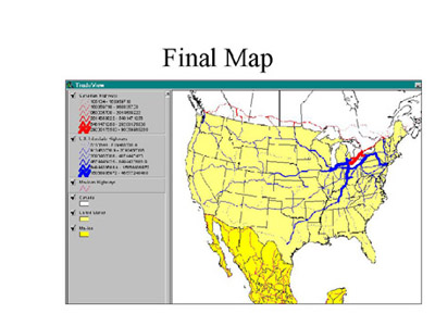
This is the shapefile now used by the avenue script to draw the final NAFTA Highway Trade Corridor Map as shown in figure 18 below. Comparison with the traditional corridor map shown earlier in this paper shows how similar this map is. However, this map can now be tailored by the non-technical user to meet individual analysis requirements. Since the trade data can be updated easily from the monthly files posted by BTS on their web site, we can maintain the currency of these maps in a very timely fashion. Transportation planners now have an easy and effective tool for monitoring the impact of NAFTA trade on the highway infrastructure of the NAFTA countries.
During the development of the trade view application several issues were raised. This was actually a goal of the first iteration of attempting to build this tool. We wanted to identify design issues and limitations so we can address them in later versions of the application and in later develop efforts. The first limitation is the state level destinations. Since we only have a single location in each state we are missing route information that might change if we had more detailed local information on the actual destination for trade. Currently, BTS only provides information at the state level. In later versions we would like to develop a method for allocating this trade to local areas within each state. This would provide more detail routing, particularly at the terminus of the trade routes. These local destinations can have a considerable impact on the routes even well before reaching the destination (or origin) state. This is particularly true of large states with either a north-south orientation (i.e. California) or an east-west orientation (i.e. Pennsylvania).
The next issue is that of legend categories or data ranges. Currently we have the code generate ranges using natural breaks based on each country individually. This results in different legend ranges for the two countries on the map. There might be better methods to perform this.
Currently we are using the Interstate Highways in the U.S. for the route system. This was convenient for the first release, however truckers probably use other routes that are not in the Interstate network. In later releases other networks will be investigated. However, clearly the size of the network will impact application performance so caution will be needed.
Currently routes are generated using the shortest path method. Given the layers we are using this is the only practical way to develop them. However, if we were able to get data such a traffic loads or drive times for each highway segment, we might, in later releases, be able to generate more realistic routes.
One of the largest issues we came across is that the BTS database has trade value for all the tables. Only a couple of tables have weight as a field. Since our application has to be consistent across all the tables, we only use the value information. If BTS were to correct this deficiency, or we could obtain a different data source, weight or truckloads would provide more meaningful corridor maps for transportation planners.
The application we were able to develop clearly had some major benefits. It is very easy to use, no GIS or programming skills are required. There is little or no training required and the application is fairly intuitive. The corridor maps produced by the application are custom tailored to individual user criteria as determined by the user selection on the query form. Users can select a single crossing, any combination of crossings or all major crossings. Users can look at a whole year's worth of trade or individual months. Users can compare month to month, same month one year to same month another year, or even season to season.
The application now provides access to timely data since we can download monthly data from the BTS web site and have it in the application in a matter of days. This data can be distributed to users on a continuous basis. Normally BTS lags by a matter of a few months of the current date.
The application produces NAFTA Trade Corridor Maps in a common format that transportation planners are used to using.
Version 1 of the application has some limitations. First, since the trade data is based on the BTS Transborder data set, there are several well-known and understood limitations associated with this data. However, many planners are well aware of these limitations and they are well documented on the BTS Transborder Surface Freight Data web site.
Also, the current version of the application supports only the selection of Canada or Mexico, Imports or Exports. Since these data sets are contained in separate tables in the BTS data, and there are slight differences in the design of these tables, it would be difficult to combine these tables to support combined queries. Work might be done to overcome this limitation in the future and allow for combined import and export trade maps and combined Canada and Mexican trade maps.
As indicated previously, the routes used in the application are to a single major destination in each state, the routes are determined by the shortest path method, and the corridors are based on $ value, not weight or number of trucks. All of these limitations are hoped to be addressed in later versions and further development efforts.
Currently the Desktop version 1 of the NAFTA Trade View System is operational. An initial user (NYS DOT in Albany) is up and running. We are currently distributing the application to other interested users. We are starting work on Web based version that would be accessible over the internet.
The next steps we plan to take in development of the Trade View Application is to collect user feedback from users of version 1. We also plan to utilize the application for a trade corridor study we are conducting as part of the NAFTA Institutes' on-going programs. We than plan to gather requests for improvements in version 2 from the users. With this feed back, we would then begin to develop version 2 of Trade View Application with enhancements.
The author would like to thank the U.S. Department of Transportation, Federal Highway Administration for the funding that supports the NAFTA Intermodal Transportation Institute and this work in particular. The author also thanks the management team at the New York State Department of Transportation that manages and administers the NAFTA Institute grant and this work in particular.