For years, engineers and scientists have been using Thiessen polygons and inverse distance squared weighting to spatially assign rainfall totals from point rain gage locations. Gage-adjusted radar rainfall can give rainfall estimates every 2 km by 2 km. and every fifteen minutes. Integration of the radar into GIS eliminates the guesswork of what is happening between the gages and has greatly improved hydrologic forecasting and water resources management.
In recent years, improvements in technology have made radar a viable tool to improve the estimation of rainfall between the gages. Radar provides a high resolution view of the variability of rain falling over a region. By merging rain data from a gage network and rain data derived from radar, hydrologists can take advantage of the strengths of each measurement system while minimizing their respective weaknesses. Essentially, a radar image is used as an areal template for the spatial distribution of rainfall. The rain gage data are used to scale the areal template. The net result is a gage-adjusted radar rainfall data set that combines the spatial distribution characteristics of the radar image with the scaling information from the gages. When input in a geographical information system such as ArcView, hydrologists and engineers can make better estimates regarding the timing, location, intensities of rainfall.
This paper will provide three examples of how GIS can be used to analyze spatial rainfall distributions that are provided with gage-adjusted radar rainfall estimates. The first example compares the different rainfall estimation procedures using both rain gages and radar. The second will look at using a specialized software package to analyze storm cell characteristics such as size, shape and direction for a ten-month study over the entire state of Florida. And the last example will focus on using HEC-GeoHMS (Doan, 2000) to create a watershed model from topographic data and using this model in conjunction with radar rainfall to create an improved hydrologic model.
The inability of rain gages to adequately resolve the spatial distribution of rainfall volume entering a watershed is why meteorologists, hydrologists, and engineers have looked to radar as an alternative tool to measure rainfall. Ever since rainstorms were first observed as noise with early military radars during World War II, hydrologists have held out hope that radar could reliably estimate rainfall accumulation (Doviak and Zrnic, 1990).
Unfortunately, for most of the past 50 plus years, radar rainfall estimates have not been accurate nor consistent enough to be useful to hydrologists and engineers. In the 1980's, as the National Weather Service planned to deploy the WSR-88D radars, it was expected that reliable radar rainfall estimation was possible (Hudlow et al., 1991). The new radars were more powerful and more sensitive than their predecessors. In addition, the new radar network was more dense, with many parts of the eastern United States covered by 2, 3, 4 or even 5 radars simultaneously.
While the WSR-88D radars represent a great meteorological success story, they have not provided the final solution to the rainfall estimation problem. It is now generally accepted that rain gages, despite their deficiencies, remain an important part of the rainfall estimation solution (Fulton et al., 1998).
Today, hydrologist have two different measurement tools to estimate rainfall, each with its own strengths and weaknesses. The strength of a rain gage is its ability to measure rainfall at a point. Its weakness is the lack of insight to what is happening in the vast areas between gages. The strength of radar is its ability to define the spatial variability of rainfall. Its weakness is its relative inability to consistently describe the absolute depth of rainfall at a given location.
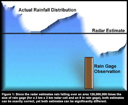
Rain gages and radars are difficult to compare directly because they measure the same physical process in two fundamentally different ways. Radar estimates the average rainfall over an area and is available in 2 km x 2 km radar pixel. Rain gages essentially sample rainfall at a point often measuring less than 0.000000028 sq mi for a 12 in diameter rain gage. The rain gage observation is a function of the gage's location within the pixel. Figure 1 shows a hypothetical example of the true distribution of rainfall along one slice through a radar pixel. The radar estimate is the average across the entire pixel but the rain gage measurement depends upon the gage's location along the slice. Both observations can be exactly correct yet both observations can be significantly different.
To demonstrate the problem of correcting radar estimates to rain gage observations, consider the situation with two rain gage observations in the same pixel. During Tropical Storm Frances in September 1998, two gages located in the same 16 sq km radar pixel measured rainfall totals that differed by a factor of two. During the storm, the radar measured an amount that was in between the estimate of the two gages (Hoblit, 1999). Since the measuring scale of a radar pixel is so much greater than the measuring scale of a rain gage, one should use caution when comparing the two estimates.
Figure 3 shows the daily summary of all the storms identified for December 29, 1998. Each 15-minute storm ellipse is shown with a motion vector and alternate colors of light and dark green distinguish ellipses for successive periods. On this day, most of the storm ellipses were quite large and elongated, a typical feature of frontal storms.
In all, 221,771 individual 15-minute storms were identified, tracked, and categorized. The histogram of storm areas is shown in Figure 4. For the study period, storm sizes ranged from a minimum of 12 sq. mi to a maximum of 9,648 sq mi, with a mean storm size of 172 sq mi. The distribution shown in Figure 4 is heavily skewed toward small storms. Fifty percent of all storms analyzed were less than 42 sq mi. Nearly 75% of all storms during the 10-month study period were less than the current density of telemetry and data recorder rain gage stations over the St. Johns River watershed. This is compelling evidence that the majority of the high intensity portions of individual storms in a given 15-minute period have a strong chance of going undetected by the existing gage network.
More in-depth information on this project can be found in Curtis (2001).
HEC-GeoHMS uses digital elevation models (DEM) to determine watershed boundaries and flow paths by analyzing the direction of steepest descent at each grid cell. DEMs are gridded topographic data that represent the elevation of a regularly spaced grid cells as the midpoint elevations of those grid cells. DEMs with 30 m horizontal resolution are available from the U.S. Geologic Survery (USGS) and were used for this analysis. In Figure 5, a hypothetical DEM (north is up) is shown with grid center elevations. Water from each grid cell will flow into one of the eight surrounding grid cells. For instance, in the northwest grid cell (elevation 59), water will flow directly to the east (elevation 56). In the grid cell immediately southeast of the original cell (elevation 58), water will either flow directly north to elevation 56, or will flow to the northeast to elevation 53. The slope to the path to the north would be (58-56)/1, or 2 elevation units per cell. The slope to the path to the northeast would be (58-53)/1.414, or 3.54 elevation units per cell. Therefore, water will flow to the northeast. In Figure 5, the grid cell with elevation 53 has a total of three upstream cells that flow into it. (Note that prior to analysis, HEC-GeoHMS creates a "hydrologically corrected" DEM, which insures that at least one of the eight neighboring cells is lower than the original cell.) An in-depth description of these processes can be found in Kull and Feldman (1998).
This analysis is completed for each cell in the DEM. At each cell, cell drainage data are determined by calculating the number of contributing upstream cells. Streams are defined when a threshold number of cells is exceeded. Cells with no upstream contributing cells form a watershed divide. Watersheds are automatically defined by HEC-GeoHMS based on user-defined threshold for watershed size and at stream confluences. The user can manually add a watershed by defining an outlet on the stream network (at the location of a gaging station, for instance), and the user can merge connected watersheds. One note of caution: Ahrens and Maidment (1999) state that the user should be "leary" of using 30 m DEMs with an average slope of less than 0.0008 (4 ft/mi or 0.8 m/km).
Figure 6 shows a watershed model created from a DEM using HEC-GeoHMS for a 160 sq mi study area near Heppner, Oregon. The watersheds were defined using a predefined threshold for watershed area, and additional watersheds were created at two gaging stations. Figure 7 shows the intersection of the radar data cells with the watershed boundary. At each cell, HEC-HMS determines the rainfall excess and routes the excess to the basin outlet based on the distance to the outlet. Using this quasi-distributed approach should be able to model complex rainfall more accurately than the standard lumped parameter models.
The preliminary modeling results for this study were mixed, but the model has yet to undergo extensive calibration and validation. Figure 8 shows the modeled and observed hydrograph response at the two gaging stations for a single storm. The model was able to capture the timing and peak at one of the stations, but performed poorly at the other station. While there is the possibility of data recording errors at the second gage, the model still needs some work.
A second study performed by the Army Corps of Engineers for the Anacostia River basin in southern Maryland had much better results. The study compared the predicted hydrograph response using the rain gages and the using the gage-adjusted radar rainfall estimates with the measured results (Figure 9). In the study, which did include a thoroughly calibrated hydrologic model, the predicted hydrologic response from the gage-adjusted radar was able to capture the timing and peak much better than the rain gage model. Obviously, more research is needed to quantify the level of improvement in the hydrologic prediction using gage-adjusted radar rainfall estimates in conjunction with a physically-based model versus using just rain gages with a lumped parameter model.
Curtis, David C. (2001). "High Resolution Radar-Rainfall Estimation in Florida." Presented at the World Water Environment Resources Conference 2001 - Bridging the Gap: Meeting the World's Water and Environmental Resources Challenges." Orlando, Florida.
Dixon, Michael and Gerry Weiner. (1993). "TITAN: Thunderstorm Identification, Tracking, Analysis and Nowcastin - A Radar-based Methodology." Journal of Atmospheric and Oceanic Technology, 10(6): 785-797.
Doan, James. (2000). Geospatial Hydrologic Modeling Extension HEC-GeoHMS - User's Manual - Version 1.0. Davis, California.
Doviak, Richard J. and Dusan S. Zrnic. (1993). Doppler Radar and Weather Observations. San Diego: Academic Press, Inc.
Fulton, Richard A., Jay P. Briendenbach, Dong-Jun Seo, Dennis A. Miller, and Timmothy O'Bannon. (1998). "The WSR-88D Rainfall Algorithm." Weather and Forecasting, 13: 377-395.
Hoblit, Brian C. (1999). "Spatial Scale Data Requirements Using NEXRAD (WSR-88D) for Accurate Hydrologic Prediction in Urban Watersheds." M.S. diss., Rice University.
Hudlow M.D., J.A. Smith, M.L. Walton, and R.C. Shedd. (1991). "NEXRAD: New Era in Hydrometeorology in the USA." Presented at the International Symposium on Hydrological Applications of Weather Radar. Hannover.
Kull, Daniel W., and Arlen D. Feldman. (1998). "Evolution of Clark's Unit Graph Method to Spatially Distributed Runoff." Journal of Hydrologic Engineering, 3(1): 9-19.
Peters, John C. and Daniel J. Easton. (1996) "Runoff Simulation Using Radar Rainfall Data." Water Resources Bulletin, 32(4): 753-760.
David C. Curtis, Ph.D.
President, NEXRAIN Corporation
E-mail: dccurtis@nexrain.com