Title
Author’s
Name
Abstract
Paper
Body
Acknowledgements
Author
Information
Food and water shortages continue to threaten populations at global scales. The inadequacy of regional transportation infrastructures to match food supply with food demand punctuate the problem.
Earth Satellite Corporation (EarthSat) of Rockville, Maryland worked with iSciences, Ann Arbor, Michigan to develop a GIS that assesses food and water balances at regional scales. Flow and iterative process models were applied to map food and water supply, demand, and balance to identify chronic problem areas globally. This paper will highlight EarthSat's GIS methods for mapping food and water balance in Africa.
The pilot GIS included ArcInfo scripted models, map databases, statistics, cartographic products and ArcView projects for all of Africa. GIS tools were also developed for complex interactive buffer zone analysis in ArcView.
A series of critical questions to be addressed though GIS process modeling were identified. The model objectives were to map the location and extent of areas of food and water surplus and shortage for 1998 for Africa, the project pilot area.
Critical questions to be addressed included identifying the location and extent of:
The project also tested model criteria and relationships to generate spatially referenced map databases as inputs for additional analysis.
Food Balance Study Area
The pilot project developed regional scale GIS models for the entire African Continent at 1 kilometer resolution. The approximate scale of use is 1:60,000,000, and datasets may be used at scales up to 1:1,000,000. All models were masked through a 8901 x 8201 1 kilometer resolution GRID.
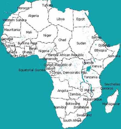 |
| Africa Study Area |
EarthSat integrated a number of publicly available spatial data sources to develop the food balance models:
Digital
Chart of the World (DCW)
International Geosphere Biosphere Programme (IGBP) Land Use/Land Cover
National Oceanic and Atmospheric Administration (NOAA) DMSP Night Time Lights,
Precipitation
US Geological Survey (USGS) GTOPO30 Elevation
United Nations Food and Agriculture Organization (FAO) FAOSTAT Database 1998,
including food production and consumption information across numerous food
types, commercial agriculture and food imports and exports
FAO Soils Database (Digitized 1995, source, 1974-78)
Food Balance Hardware and Software
EarthSat used commercial off the shelf GIS software to implement the pilot project. Software included ArcInfo 8 GIS, ArcView 3.2 Desktop GIS, and Erdas Imagine 8.4 Image Processor. ArcInfo GRID was the primary analytical software tool. Hardware included a Dual Xeon 500s NT PC client running SCO Xvision, and a SUN Enterprise 4000 Solaris server.
Food Balance Findings and Methods
Earthsat developed a supply/demand and balance approach to estimating regional food balance in Africa. A demand surface is subtracted from a supply surface to produce a food balance surface showing areas of food surplus and shortage. The food balance surfaces are based on figures contained in the Food and Agriculture Organization of the United Nations’ FAOSTAT database for 1998, the most current period that was available.
Food Supply
The food supply surface shows total food available, expressed in daily calories, per square kilometer. Supply is the total estimated calories for human consumption from domestic production and food imports. Since FAOSTAT data estimates commercial agriculture production, the food supply surface does not account for noncommercial agricultural production, such as subsistence agriculture.
Food Imports
The food imports surface is an allocation of national food import caloric estimates to a 1 kilometer resolution suitability surface. Suitability for food import allocation is based on cost distance from major import centers, such as port cities, population density, and a weighted concentration of wealth surface.
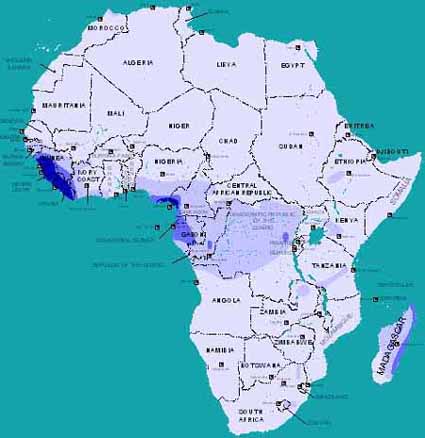
Food imports are derived by allocating FAOSTAT national estimates of 1998 food imports to an enhanced suitability surface. First, food import centers are identified. Major import locations are created from the CIA World Factbook and evaluation of 1998 ORNL population density, and DCW transportation infrastructure (major rail and road junctures).
Next, a friction surface is produced that represents the cost of transporting food from import centers to demand areas. The friction surface assigns low cost to transportation infrastructure areas. High population density areas also receive a low cost designation. This reflects the economy of scale of supplying food to high population density centers. This friction surface is used to generate a cost distance surface from import centers. This surface shows the cumulative weighted distance of providing food from import centers. The cost distance surface is inverted to derive a suitability surface. The resulting surface shows the suitability of the landscape for food imports.
 |
| Africa Cost Distance from Import Centers |
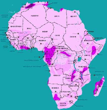
Before the suitability surface is created, the cost distance surface is modified by two factors. First, population density is applied to reduce cost distance. 1998 ORNL population is proportionally adjusted to tie to 1998 FAOSTAT national population totals. The cost distance surface is reduced proportionally to population. Highest population density areas receive greater cost reductions, while lower density population centers smaller cost reductions. This fosters allocation of food supply to heavy food demand areas.
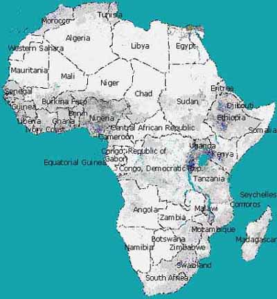 |
| ORNL Africa Population Density 1998 |
Second, a wealth factor is applied to the cost distance surface. This wealth factor uses GINI concentration of wealth estimates as well as disaggregated wealth to concentrate food in areas of higher wealth, and reducing food concentrations in areas of lower wealth. The GINI factor modifies the influence of wealth on the costdistance surface. Thus, in areas of higher GINI coefficients (reflecting higher concentration of wealth), the impact of wealth is stronger on the allocation of food imports. Conversely, in areas of lower GINI coefficients (reflecting more even distributions of wealth), the impact of wealth is weaker on the allocation of food imports.
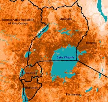
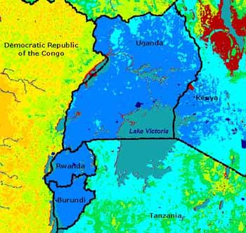 |
| Lakes Region Disaggregated Wealth |
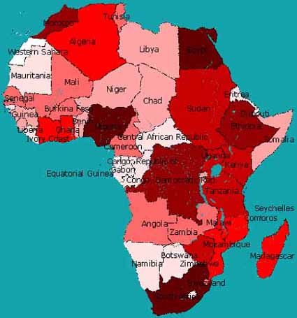
 |
| UNDP National GINI Indicators |
Population density and wealth are thus factored into cost distance to produce a suitability surface for food imports. In this surface, areas of high population density, high wealth, and low cost distance to food import centers will experience greater concentrations of food imports. Conversely, low density, isolated, lower wealth areas will experience lower concentrations of food imports.
National food imports (daily calories) from the 1998 FAOSTAT database are allocated to the suitability surface to map a food import surface (total daily calories).
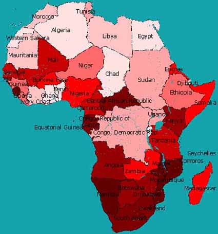
 |
| Africa National Food Imports 1998 |
 |
| Africa Allocated Food Imports, Total Calories Per Square Kilometer |
Domestic Food Production
The domestic food production surface shows the total daily calories available for food consumption from domestic production. Agricultural primeness (the suitability of the landscape for agricultural use) and a proximity to agricultural primeness surface is combined with disaggregated wealth and 1998 population density to model a distributed domestic food supply surface.
The agricultural primeness surface is the suitability of the landscape for agricultural use. The agricultural primeness model uses two compound weighted criteria (physical and socio-economic factors) to index suitability in a raster surface:
1. Physical Characteristics
These layers are modeled to reflect the physical characteristics of the landscape that favor agriculture. The three component criteria are soils, moisture availability and landcover. The criteria are :
a.
Moisture Availability.
Average annual rainfall
Access to streams (based on a cost surface)
b.
Soil Suitability
Soil type/agricultural productive potential
Slope
 |
| Lake Region FAO Soils 1974-78 |
c.
Land Cover
Land cover type suitability for agricultural use. For example, agricultural
areas received higher suitability scores for agricultural use than barren
land and open water areas.
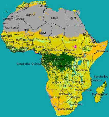 |
| Africa IGBP Land Use/Land Cover 1992-93 |
2. Socio-economic Characteristics
A single socio-economic layer that represents access to demand centers for agricultural products was produced. This surface assigns high agricultural primeness scores to areas which have easy access to higher density population centers, and lower agricultural primeness scores to areas that have poor access to low density population centers :
a.
Access to demand for agricultural products.
Access to settlements (agricultural demand centers) (based on a
slope-derived cost surface)
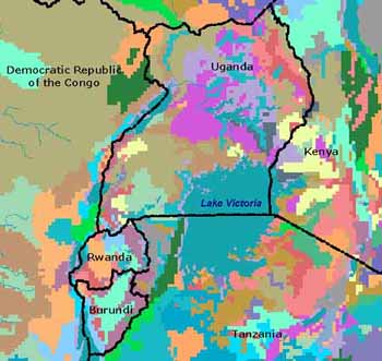
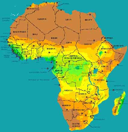
 |
| Lakes Region Agricultural Primeness |
To distribute food supply from the point of production to the point of demand, additional proximity, wealth, and population density criteria are applied. The proximity criteria charactierizes the 'nearness' of the landscape to areas of high agricultural primeness. Areas that are closest to areas of high agricultural productivity receive an increase in suitability for domestic food supply. Areas that are distant to centers of high agricultural productivity are assigned a lower suitability score than areas nearby.
The wealth criteria serves a similar purpose as in the food import component. The wealth factor uses GINI estimates as well as disaggregated wealth to concentrate food in areas of higher wealth, and reducing food concentrations in areas of lower wealth. The GINI factor modifies the influence of wealth on the costdistance surface. Thus in areas of higher GINI coefficients (reflecting higher concentration of wealth), the impact of wealth is stronger on the allocation of domestic food supply. Conversely, in areas of lower GINI coefficients (reflecting more even distributions of wealth), the impact of wealth is weaker on the allocation of domestic food supply.
Lastly, 1998 ORNL population density, adjusted to tie to FAOSTAT population estimates is used to concentrate domestic food supply. Higher density population areas receive greater suitability for domestic food supply than low population density settlements.
These agricultural primeness, proximity to agricultural primeness, wealth, and population density criteria are combined to develop an aggregate domestic food supply suitability surface. 1998 FAOSTAT national domestic food production (daily calories) are then allocated to the aggregate suitability surface to derive a domestic food supply surface (total daily calories).
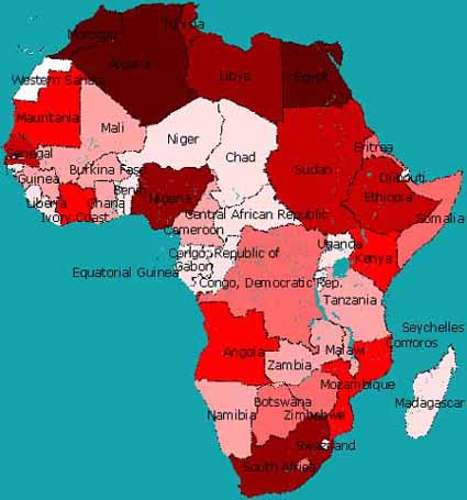
 |
| Africa National Domestic Food Production, 1998 |
 |
| Distributed Domestic Food Production |
The total food supply surface is the sum of food imports and domestic food supply. It shows the total available food supply in daily calories from commercial agriculture, from imports and domestic production.
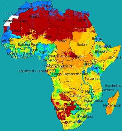
 |
| Africa Total Food Supply |
Two food demand scenarios are developed. The first scenario uses 1998 FAOSTAT national averages for daily caloric consumption. The national average food consumption is weighted by adjusted 1998 ORNL population density to develop a surface of food demand (average daily calories). The 1998 ORNL population is adjusted to match 1998 FAOSTAT figures for population totals.
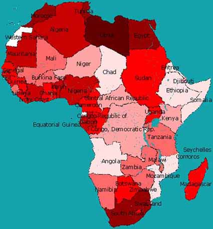 |
| Africa National Average Daily Caloric Consumption Per Capita 1998 |
|
| Africa ORNL Population Density Per Square Kilometer, 1998 |
 |
| Africa Food Demand, National Average Caloric Demand |
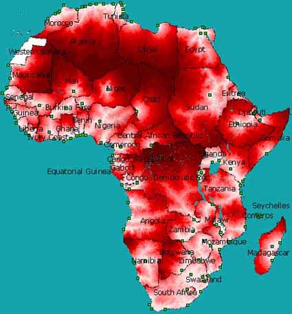
The second food demand scenario uses an average food consumption of 2,000 calories per day per person to generate a food demand surface.
 |
| Food Demand, 2,000 Calories Per Day Per Capita |
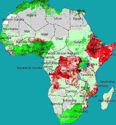
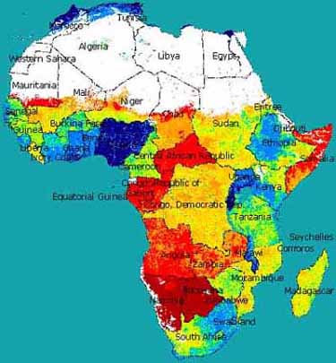
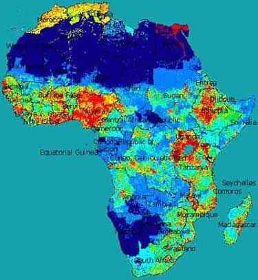
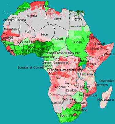
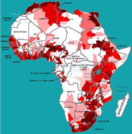
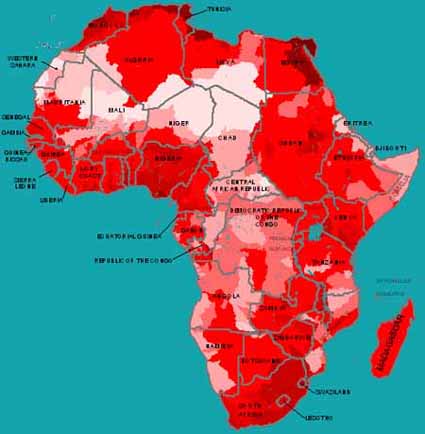
Food balance is the aggregate difference between food supply and demand. The surface shows areas of food shortage and surplus throughout Africa, in total daily calories. Two scenarios are produced which present differing demand components. The first scenario models food balance based on 1998 national averages for daily caloric consumption.
 |
| Food Balance, National Average Daily Caloric Consumption |
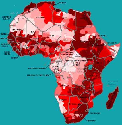
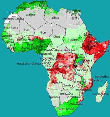 |
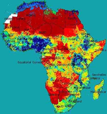
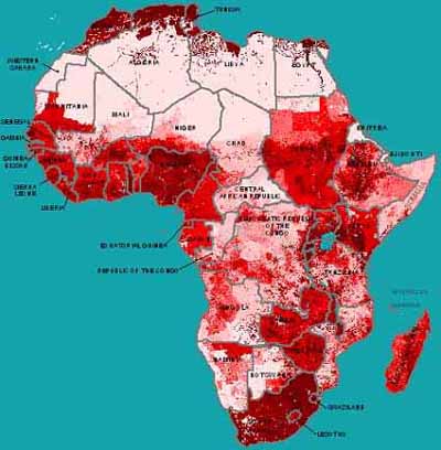
| Africa Food Balance, 2000 Calories Daily Consumption Per Capita |
The maps illustrate how 2,000 calories per day represents an actual increase in caloric consumption for many African states. The map highlights areas which could experience food shortage in the event that all people consumed 2,000 calories daily, per country.
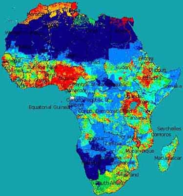
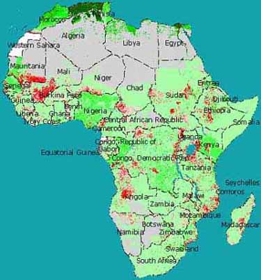
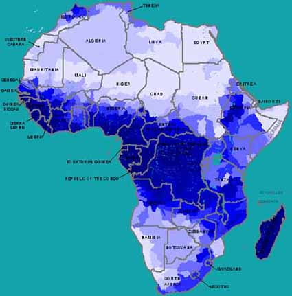
EarthSat also developed food balance scenarios showing the impact of disruption of food imports. The maps show food balance where total food supply is based only on domestic production.
 |
| Food Balance, No Food Imports, National Average Caloric Consumption |
The map database showing food balance without food imports, based on national average caloric consumption illustrates the magnitude of sensitivity of areas to food import interruption.
 |
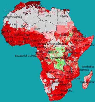
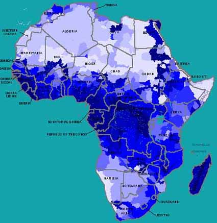
| Food Balance, No Food Imports, 2000 Calories Daily Per Capita Consumption |
The
map databases showing food balance without food imports, at 2000 calories
daily consumption, in particular shows areas that could mitigate interruption
of food imports by reducing food consumption to 2,000 calories per capita per
day.
Food Balance Recommendations for Further Work
The Africa Food Balance surface will benefit from additional effort including observational information for the purpose of model calibration. The inclusion of food production from urban gardens and subsistence agriculture will provide a more complete picture of African food supply. As more current data is made available, time series will be possible for longitudinal studies, and for forecasting.
Work is in progress to develop the food balance models for the South Asian continental region.
EarthSat also developed a supply, demand, and balance modeling approach to mapping renewable water resources. The Africa water balance GIS model draws total average annual water demand from total average annual renewable water supply to estimate a regional scale watershed water balance. The GIS addresses critical analysis questions, identifying by watershed throughout Africa the location and extent of:
Renewable
Water Supply
Water Demand from industrial, agricultural and domestic sectors
Water surplus and shortfall throughout the continent
The dependency of watersheds on inflow from exterior watersheds to meet local
water demand
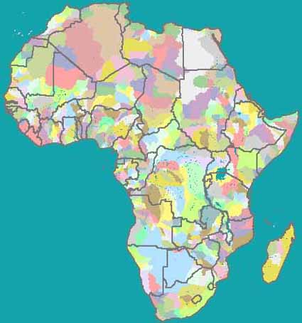
The pilot project developed regional scale GIS models for the entire African Continent at 1 kilometer resolution. The approximate scale for use is 1:60,000,000, and datasets may be used at scales up to 1:1,000,000. All models were masked through a 8901 x 8201 one-kilometer resolution GRID. Results were aggregated to US Geological Survey (USGS) HYDRO1K Level 3 watersheds for regional scale analysis.
|
| Africa Water Balance Study Area, USGS HYDRO1K Level 3 Watersheds |
Renewable water supply is derived from Esri ArcAtlas 'Our Earth' groundwater discharge and runoff, and National Oceanic and Atmospheric Administration National Geophysical Data Center precipitation and evapotranspiration 1931-1960.
 |
| Africa Surface Runoff, Esri ArcAtlas |
 |
| Africa Groundwater Discharge, Esri ArcAtlas |
The groundwater discharge layer is produced by weighting NOAA precipitation by the Esri ArcAtlas groundwater discharge coefficient surface.
 |
Evapotranspiration is subtracted from total precipitation, runoff and groundwater discharge to estimate total renewable water supply per square kilometer and by Level 3 Watersheds.
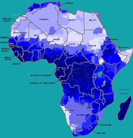 |
| Africa Total Water Supply, Level 3 Watersheds |
Water demand is derived from World Resource Institute (WRI) 1998 estimates of national water consumption for industrial, domestic and agricultural sectors. These sectors were mapped using NOAA DMSP night time lights and International Geosphere Biosphere Programme 1 km land use/land cover map databases, and the ORNL 1998 Landscan Population density product.
 |
| Africa Industrial Water Demand, Level 3 Watersheds |
Areas of persistent night time bright lights were identified to model industrial areas. These areas were modeled as industrial water demand centers.
 |
| Africa Agricultural Water Demand, Level 3 Watersheds |
IGBP Land Use/Land Cover cropland and cropland/natural mosaic landcover areas were modeled as agricultural water demand centers.
 |
| Africa Domestic Water Demand, Level 3 Watersheds |
ORNL 1998 population was weighted by WRI national water consumption estimates to map domestic water demand.
 |
| Africa Aggregate Water Demand |
Total water demand is modeled as the sum of industrial, agricultural and domestic water demand.
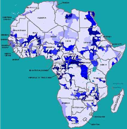
A static water balance, showing water surplus and shortage without consideration of interwatershed flow is produced. Total water demand is subtracted from total water supply to derive static water balance.
 |
| Africa Static Water Balance, Level 3 Watersheds |
Next, interwatershed flow is modeled to produce an end-state water balance. The connectivity of watersheds is identified, and intershed water flow is programmed in a process GIS model. Throughout the course of flow, water balance is drawn down by local demand. End-state water balance shows water shortage and surplus where water has flowed through the drainage network and reached its final destination. Surfaces showing water supply, demand and balance normalized for watershed area were also produced. The surfaces addresses the critical question of identifying the location and extent of water supply, demand and balance at a regional watershed level.
 |
| Africa End-State Water Balance, Level 3 Watersheds |
The total volume of water inflow to each watershed is also identified to show upstream dependency from exterior watersheds for water supply.
 |
| Africa Upstream Watershed Dependency, Level 3 Watersheds |
Water Balance Recommendations for Further Work
The Water Balance surface will also benefit from additional model calibration based on observational data. While manual techniques for identifying interwatershed flow are time consuming, no reliable and accurate fully computer automated techniques for correctly producing interwatershed flow exist. It remains more time-effective to manually identify watershed connectivity, and code the relationships into a database. As with food balance, as more current data is made available, time series will be possible for longitudinal studies and forecasting.
Water balance modeling is also in progress for the South Asian continental region.
ArcView 3.2 Tools
EarthSat developed a series of ArcView 3.2 supporting analytical and distribution/packaging tools. The tools simplify buffer zone analysis and allow endusers to automatically package the spatial data sets into uniform user-selected extents. A buffer analysis tool allows endusers to conduct complex buffer and zonal analysis. For instance, end users may buffer a feature, such as a stream or latitude/longitude coordinate, and rapidly characterize any GRID surface within that buffer zone (such as summarizing average food balance). A clipping tool assists in production of project packaging. For instance, end users may rapidly extract all model layers for a specific country, rectangular extent, geographic latitude/longitude extent, or buffer zone extent.
The author wishes to acknowledge Douglas Way and Ric Cicone of iSciences for their direction and Michael Blank and Christopher Schierkolk of EarthSat for their assistance in implementing this GIS project.
Jeffrey
B. Miller
Staff
Scientist
Earth
Satellite Corporation
6011
Executive Boulevard, Suite 400
Rockville,
MD 20852-3804
jmiller@earthsat.com
http://www.earthsat.com