- An agrichemical distribution database was created as part of an EPA Ecosystems Indicators
Project for the purpose of evaluating effects of multiple stressors on agriculturally impacted
wetlands. USDA Farm Service Agency data, including crop type and acreage, were collected
and used to generate the database with all data aggregated into Public Land Survey (PLS)
sections (nominally 1 square mile). Mapping and modeling of agrichemical distribution, inferred
from crop type, acreage, and normal agrichemical application rates, has enabled researchers to
select PLS sections with specific combinations of agrichemical stressors and potentially
impacted wetlands.
As part of an EPA funded Ecosystems Indicators Project designed to evaluate the effects of multiple stressors on agricultural wetlands, it was necessary to characterize in significant detail the agricultural practices for the study area. The types of information needed included wetlands, crops and acreage planted, location of planted crops, and agrichemical application rates and practices. The area of study is the Little Tallahatchie River drainage basin in northern Mississippi (figure 1). The basin encompasses an area of approximately 2000 square miles and is contained in parts of nine different counties.
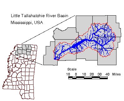
FIGURE 1: Location Reference
The aggregated data could not be used to characterize the agricultural practices in the
basin for several reasons. There are only nine data points, representing the nine counties, with
which to characterize the basin. The data would represent a whole county, whereas the study
basin only represented a fraction of the area of the county. Finally, agricultural practices vary
significantly throughout the basin, dependent on topography and geology; in some cases the
agriculture represented by the county numbers might not even be in the basin.
The scope of the project included an evaluation of the combined effects of the chemicals; characterization of the basin sought to identify sites in which the given chemicals might occur in specific combinations. The primary criterion for choosing a wetland site for sampling was the likelihood that the site might be affected by specific agricultural practices. This project is investigating potentially interacting stresses caused by four commonly used chemicals: Methyl Parathion, Clorpyrifos, MSMA, and Atrazine.
To more accurately characterize the basin, farm data was obtained from the local county Farm Services offices located in each county. The farm data contained the following key items:
The PLSS location reference contained on the data sheets for each farm tract provided the means to spatially locate the reported agriculture practices. The PLS System is a common land survey system used through most of the U.S. In consists of a series of north-south trending Meridians and east-west trending Base Lines. These Meridians and Baselines are the used to reference columns and rows called Townships and Ranges, each having a width of 6 miles. Each Township and Range cell or block is composed of 36 Sections each 1 square mile. The legal definition of land location using the PLSS system can further divide the Sections into quarters or other fractional unit. The PLSS location reference for each farm tract was to the nearest section, effectively giving researchers a spatial location accurate to within one square mile. Agricultural characterization of the basin was completed based on the PLSS grid (nominally one square mile) increasing the number of data points to over 2000.
The farm and tract data was collected from each of the nine county Farm Service offices for each PLSS section contained in the study basin. Data was then entered into a database with attributes linked to a unique identifier created by the farm tract number and a code for each county. Using the sum feature provided by ArcView (Esri), data was aggregated into total values for each of the PLSS sections in the basin. The resulting data set provided a more detailed description of the distribution of the agriculture crops planted across the basin. Figure 2 shows the distribution of Cotton acreage for the study basin.
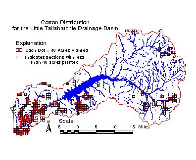
FIGURE 2: Example Crop Distribution map
The scope of the project included an evaluation of the combined effects of the chemicals; characterization of the basin sought to identify sites in which the given chemicals might occur in specific combinations. The primary criterion for choosing a wetland site for sampling was the likelihood that the site might be affected by specific agricultural practices. This project is investigating potentially interacting stresses caused by four commonly used chemicals: Methyl Parathion, Clorpyrifos, MSMA, and Atrazine.
To more accurately characterize the basin, farm data was obtained from the local county Farm Services offices located in each county. The farm data contained the following key items:
-
Identification numbers - which could be used to cross reference data from
previous years as well as provide a unique identifier (consisting of a farm
and tract number
- Type of crop planted and acreage planted
- Public Land Survey System (PLSS) location for the farm
The PLSS location reference contained on the data sheets for each farm tract provided the means to spatially locate the reported agriculture practices. The PLS System is a common land survey system used through most of the U.S. In consists of a series of north-south trending Meridians and east-west trending Base Lines. These Meridians and Baselines are the used to reference columns and rows called Townships and Ranges, each having a width of 6 miles. Each Township and Range cell or block is composed of 36 Sections each 1 square mile. The legal definition of land location using the PLSS system can further divide the Sections into quarters or other fractional unit. The PLSS location reference for each farm tract was to the nearest section, effectively giving researchers a spatial location accurate to within one square mile. Agricultural characterization of the basin was completed based on the PLSS grid (nominally one square mile) increasing the number of data points to over 2000.
The farm and tract data was collected from each of the nine county Farm Service offices for each PLSS section contained in the study basin. Data was then entered into a database with attributes linked to a unique identifier created by the farm tract number and a code for each county. Using the sum feature provided by ArcView (Esri), data was aggregated into total values for each of the PLSS sections in the basin. The resulting data set provided a more detailed description of the distribution of the agriculture crops planted across the basin. Figure 2 shows the distribution of Cotton acreage for the study basin.
FIGURE 2: Example Crop Distribution map
Agrichemical usage data was then generated from accepted application rates for each
crop type combined with acreage of the crops planted. Application rate data was obtained
from local County Extension offices. An example would be – section XX had 200 acres of
cotton planted, with an MSMA application rate of 2.53 kg/acre for cotton yields and expected
chemical loading of 506 kg could be expected for that section. The total amount for each of the
chemicals was then divided by the area of the section (acres). If section XX were of the
nominal 1 square mile (640 acres) then the loading rate for the section would be 0.79 kg/acre.
Figure 3 is a map of the usage of MSMA for the study basin. The final step served to normalize
the chemical data by the area of each section. This was necessary because the actual PLSS
grid has some inconsistencies resulting in sections that are not of the nominal size. The best
example of this occurs in the western portion of the study basin, where the PLSS grid is reset
along a northwest-southeast trending line - an old Indian treaty boundary (figure 4).
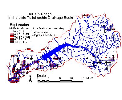
FIGURE 3: Example Chemical Distribution Map
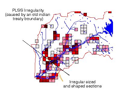
FIGURE 4: Example of PLSS Irregularity
FIGURE 3: Example Chemical Distribution Map
FIGURE 4: Example of PLSS Irregularity
A ranking of NONE, LOW, or HIGH chemical loading was assigned to each section
for each of the given chemicals, based on the maximum loading for a given chemical in any
section in the basin. A value of NONE was assigned to sections with no expected usage of a
chemical. A Value of LOW was assigned to sections with an expected usage of less than 25%
of the maximum. HIGH was reserved for sections with expected usages exceeding 25% of the
maximum. Using a simple technique of assigning a numerical value for each rank, a composite
of the total chemical loading was created. For instance the NO, LOW, or HIGH ranking for
MSMA was assigned to single digits (i.e. 1, 2, or 3), where as, Atrazine was assigned to double
digits (i.e. 10, 20, or 30). When simply added, the resulting number represents the ranking of
the four chemicals for the given sections. An example would be 2321: Methyl Parathion – low
ranking (2000), Chlorpyrifos – high ranking (300), Atrazine – low ranking (20), and MSMA –
none present (1).
Figure 5 illustrates the distribution of potential agrichemical combinations in the Tallahatchie River Basin by section. This compilation of FSA data allowed researchers to locate sections with specific chemical combinations to be able to study the effects of multiple stressors. From these data, sections were selected to locate wetlands for sampling. The GIS database contains the necessary information for biologist to be able to evaluate the results of biological testing of wetland ecosystems.
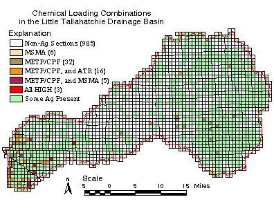
FIGURE 5: Completed Chemical Distribution Map
Figure 5 illustrates the distribution of potential agrichemical combinations in the Tallahatchie River Basin by section. This compilation of FSA data allowed researchers to locate sections with specific chemical combinations to be able to study the effects of multiple stressors. From these data, sections were selected to locate wetlands for sampling. The GIS database contains the necessary information for biologist to be able to evaluate the results of biological testing of wetland ecosystems.
FIGURE 5: Completed Chemical Distribution Map
ACKNOWLEDGEMENTS:
University of Mississippi – Oxford, Mississippi
Project: EPA/NCERQA Ecosystems Indicators Program: EPA Award R826595-01-0
Project Coordinator: Dr. Stephen T. Threlkeld (Email: stt@olemiss.edu)
Project Web Page: http://www.olemiss.edu/projects/epa-eig
AUTHOR INFORMATION:
Harold D. Robinson Jr.
Graduate Student/GIS Technician
University of Mississippi
Department of Geology and Geological Engineering
118 Carrier Hall
University, MS 38677
Phone: (662) 915-7498 – Dept.
Email: HRobin1499@aol.com
Dr. Greg Easson, Associate Professor
Director, University of Mississippi Geoinformatics Center (UMGC)
University of Mississippi
Department of Geology and Geological Engineering
118 Carrier Hall
University, MS 38677
Phone: (662) 915-5995 – Office
Email: geasson@olemiss.edu
Dr. Stephen T. Threlkeld, Professor
University of Mississippi
Department of Biology
318 Shoemaker
University, MS 38677
Phone: (662) 915-5803
Email: stt@olemiss.edu