Abstract
Beyond TM: Making High Resolution Imagery Work for Urban Applications
Recent advances in digital airborne sensors and satellite platforms make accurate, high-resolution multispectral imagery readily available. This opens the door to a host of new applications to address and solve old problems. However, traditional classification and application methods are often inadequate to produce useful information products from these new data sources. High-resolution imagery is particularly well suited to urban applications. Previous data sources (such as Landsat TM) did not show the spatial detail necessary to provide many urban planning solutions. An important urban application that is now possible due to the availability of high resolution data is stormwater managment. This paper will provide an overview of the new techniques developed to create an accurate map of pervious/impervious surfaces from high-resolution imagery for the City of Scottsdale, AZ. A key component of developing techniques for new data is determining the level, and requirements, of integration with GIS. This paper will review the opportunities and issues involved with integrating these new data sources, and analysis techniques, with the developing ArcView platform.
Stormwater runoff and flooding are responsible for loss of life and billions of dollars in property damage each year. Planning and construction of drainage infrastructure to protect against or minimize these losses is a major budgetary expense shouldered by taxpayers in communities all across the nation. As part of any modern drainage infrastructure plan, engineers and planners rely upon standardized hydrologic models to estimate peak flood flows and the volume of runoff in order to plan and design drainage and flood control facilities at specific locations within defined drainage basins.
One of the most commonly used hydrologic models in the United States is the HEC-1, a product of the US Army Corps of Engineers. This program requires a number of input parameters, among the most sensitive are rainfall amount and the amount of impervious area within a given watershed. The output is the computed peak flow (“Q”) at a specified point within the watershed. This “Q” is the critical input parameter in the design and ultimate size of drainage infrastructure such as channels, storm sewer systems, culverts and bridges.
Given the high cost of building new facilities or upgrading inadequate existing facilities, it is imperative that inputs to HEC-1 be as accurate as possible. Whereas it is relatively easy to estimate probable rainfall amounts from historical records, the determination of impervious landcover percentages is not as easy and has typically been derived from nationally standardized lookup tables based on existing or projected land use classifications. Such tables may not provide the level of accuracy desired to properly define the drainage characteristics at a particular location, leading to the under- or over- sizing of drainage and flood control facilities. In the case of undersizing, the health, safety, and welfare of the public may be put in jeopardy. On the other hand, if facilities are over designed then valuable tax dollars are being wasted.
The amount of impervious surface area is by far the single most important factor affecting the amount of runoff in the urban environment. The City of Scottsdale, Arizona (COS) wanted to see if remote sensing could provide a cost-effective way to more accurately estimate this key input parameter. The City tried a different approach to the determination of impervious landcover percentages via the classification of high-resolution multi-spectral imagery using standard remote sensing processing techniques in conjunction with data from its Geographic Information Systems (GIS) database. The goal was three-fold if the remote sensing procedures proved accurate and reliable: 1) to determine actual impervious area in fully developed portions of the city, 2) to validate or correct the look-up table values for improving estimates of future conditions in the undeveloped portions of the city, and 3) to create a cost effective procedure that could be used periodically to update and correct the City’s hydrologic models as development occurs. This report will explain the background, processes, and results of the project.
Scottsdale initially partnered with Arizona State University, Tempe in 1995 to look at the possibility of developing urban applications for remote sensing data. Images from both commercially available space platforms and NASA airborne sensors that span visible to radar wavelengths were obtained and evaluated. Initially, three applications were identified as having the greatest immediate need or potential. They were: 1) environmental monitoring of the McDowell Mountain Preserve area, 2) incident mapping of the Rio fire in the northern part of the city (the largest wildland fire in the history of Arizona), and 3) stormwater management where the percentage of impervious surfaces within a sub basin would serve as a direct input into the HEC-1 hydrologic model.
Of these three applications, Scottsdale decided to emphasize the stormwater application. Airborne NASA NS001 data at 3m ground sampling distance (GSD), along with SPOT multi-spectral (20m GSD) and Landsat TM (25m GSD) images were initially used for the project. The original study area consisted of a four square mile area in the older, more developed southern part of the city.
From that initial pilot study, it was determined that in order to achieve a higher classification accuracy within a basin, other remote sensing products delivering higher spatial resolution were needed. The study area was also expanded to include a more diversified land use. The new project area includes the entire contiguous portion of the city south of the Central Arizona Project (CAP) canal. This area encompasses approximately 50 square miles. Within this region, 31 major drainage basins have been identified.
In the summer of 1999, Hammon, Jensen, Wallen & Associates Inc.(HJW) (Oakland, CA) collected airborne data with the ADAR 5500 multi-spectral digital camera system over this area at one to two meter GSD resolution. They conducted the initial post processing that involved band co-registeration, removal of vignetting effects, and geometric correction. Individual images were then mosiacked together. Pacific Meridian Resources (PMR) of Emeryville, CA was then contracted to classify the imagery and perform the accuracy assessment. The final two-class (impervious/pervious) image was analyzed in-house at the sub basin level and the results were compared to the values derived from the lookup tables.
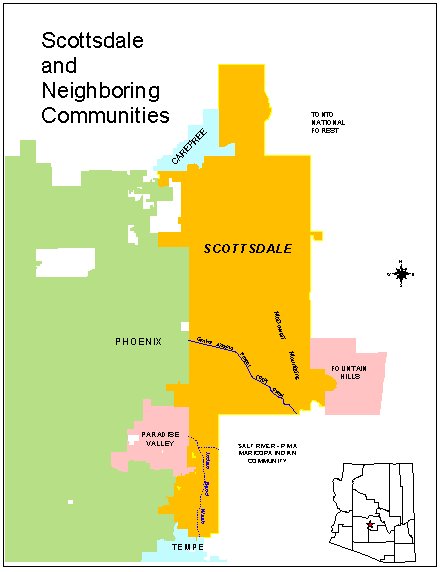
Scottsdale is located in Maricopa County, Arizona, just east of Phoenix in the south-central part of the state. The city occupies an area of approximately 185 square miles stretching 31 miles from north to south (Figure 1). Elevations rise gradually from about 1,200 feet in the south near the floodplain of the Salt River to over 4,000 feet in the north. On the eastern border are the McDowell Mountains that rise to just over 4,000 feet. Large, coalescing alluvial fans flank both sides of this north-south trending range.
Incised drainages high on the western flank (the Scottsdale side) of the mountains spread their discharge out across a broad alluvial plain as the washes flow towards the southwest. The Central Arizona Project (CAP) Canal, constructed in the 1970’s by the U.S. Bureau of Reclamation, physically subdivides the city. North of the CAP are large expanses of natural as-of-yet undeveloped desert land. On the north side of the canal is an earthen dike and retention storage basins. The dike was constructed to protect the CAP Canal from flooding. The canal delivers a major part of Arizona’s water from the Colorado River. Most of the runoff north of the CAP is retained in retention basins behind the dike. Most of the area south of the CAP is fully developed and the remaining vacant parcels are rapidly developing. The majority of the area drains into Indian Bend Wash, which bisects the southern portion of the city as it flows southward through the adjacent city of Tempe into the Salt River.
Scottsdale lies on the northern fringe of the Sonoran Desert. The climate is characterized by two distinct rainy seasons. The first occurs during the winter months of December, January, and February. Frontal storms sweep across the area from the west bringing widespread precipitation that is generally of low intensity and long duration, and may last for several days.
Contrasted with that is the summer “monsoon” season that begins in July and ends in mid to late September. Convective storms occur when moist air from the Gulf of Mexico drifts northward and eastward into the state. Precipitation from these events is localized and often high intensity and short duration. However, they are responsible for the major flood events that occur within the city.
Historical records show that the average annual precipitation can range from 7 to 15 inches. Average annual rainfall is 7.6 inches. Temperatures average from 41-66şF in the winter to 80-105şF in the summer.
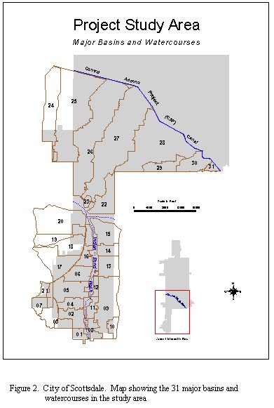
The study area is the portion of Scottsdale located south of the CAP. It was divided into 31 major drainage basins (Figure 2), which were further subdivided into 995 sub basin drainage areas, and the Indian Bend Wash, in the preparation of a Storm Water Master Plan prepared for the city in 1996. The U.S. Army Corps of Engineers, in cooperation with the City and the Flood Control District of Maricopa County, transformed Indian Bend Wash into a greenbelt area consisting of recreational facilities and retention basins. It is a major flood control channel into which most of the major basins flow and therefore was not included among the basins in this study.
Residential building practices change from south to north across the city and reflect evolving trends in housing. Generally speaking, in the older neighborhoods to the south, one finds asphalt-roofed homes situated on small lots. Most homes have grassy lawns with well established trees of introduced species not native to the Sonoran Desert.
Houses tend to have clay tile roofs and desert landscaping is more prevalent. Most of the newer homes have swimming pools. Many neighborhoods are built around greenbelt areas, golf courses, or man- made lakes that serve as stormwater retention basins.
Commercial development is centered along major thoroughfares in the southern part of the study area. In the newer areas in the north, businesses have clustered around Scottsdale Airport, large real estate developments such as McCormick Ranch, and alongside the newly built Pima Freeway.
A summary of land uses in the project area is shown in Table 1. The area, including the Indian Bend Wash, is divided into 18 landuse categories, with almost 59,000 property parcels ranging in area from less than 100 ft2 to 11,512,495 ft2, containing over 63,000 roofed structures. Nearly 40% of all dwelling units reside on Ľ-1 acre of land.
The following section describes the acquisition and processing of the remote sensing data. As mentioned above, HJW was selected through an RFP process to acquire the data and perform some initial processing steps. Scottsdale then contracted with PMR to classify the data and assess its accuracy
The mission was flown on July 17, 1999 with the acquisition of imagery occurring between ±2 hours of local solar noon. The contractor was asked to fly in one consistent direction--either south to north or vice versa—but chose instead to fly in a loop. At an altitude of 7,000’, this produced 283 digital frames arranged in 13 flight lines. These parameters were necessary in order to minimize shadow effects, have relatively stable and consistent atmospheric conditions, and a constant illumination angle. Leaf-off condition was deemed negligible for the desert environment.
The imagery was flown with a sidelap of 30% and a forward lap of 30%. This was to ensure that the optimum central portion of each frame would be available for the digital mosaic.
The four images were co-registered. Vignetting effects produced by the digital cameras were removed. Specific and recognizable features within each ADAR frame were then correlated to Scottsdale’s reference digital orthophotographs (D.O.) to closely position the frames to their true ground location. Approximately 25 control points were manually selected between each ADAR frame and the D.O
An image-to-image rectification program was then applied to each frame to digitally warp the ADAR to the D.O. This program automatically searched for up to 500 control points per frame. Once each frame was tied to the D.O., a mosaicking program was applied that selected the optimum area of each frame, tied frames together minimizing misalignments, and digitally feathered seams. The entire mosaic was evaluated for statistical x, y accuracy to the D.O.
PMR was charged with conducting the classification and its accuracy assessment along the following specified guidelines. First, the landcover classes were established as: rooftops and pavement (impervious surfaces), and bare ground, vegetation, and water (pervious surfaces). The water class included swimming pools, as well as canals. Although these features are technically impervious, they do serve to retain precipitation and thus act as pervious surfaces during storms.
Second, once the imagery was classified as far as possible into these five groups, any remaining confused pixels could be classified with the aid of ancillary GIS data. The five classes would then be collapsed into a binary image and the accuracy assessed.
Third, PMR was tasked with achieving an overall classification accuracy of at least 80% in each basin when compared to percentages of imperviousness calculated from relevant aerial photos or actual ground- truth. Additionally, producer’s and user’s accuracies of >80% would be obtained for each of the separate landcover classes
Finally, although the exact types of classification procedures to be used were left up to the contractor, the end result had to be a Windows NT ERDAS Imagine derived solution. This was to insure that the process would be repeatable and non- proprietary.
The first step in the data processing was an initial unsupervised ISODATA classification of 50 classes. The resulting image was then labeled based upon prior knowledge of the study area and 1.5 foot resolution digital ortho-photos as reference.
After this initial classification, PMR sent two people to the study area to establish field sites. Field site designation served two roles in this project: as locations for training signature creation and for determination of accuracy assessment sites. For each of the five classes, they obtained a minimum of 30 training sites and a minimum of 50 accuracy assessment sites. The field sites were assigned to either a training site coverage or an accuracy assessment coverage according to the following ratio: 1/3 for training site data, 2/3 for accuracy assessment. Landcover class using a random number generator for each polygon performed the assignations. The accuracy assessment coverage was set aside until the classification was completed and accuracy assessment was performed. This insured that the accuracy data were completely independent of the training data.
PMR then performed a Maximum Likelihood supervised classification on the data. The result of the supervised classification was entered into a statistical software program (SAS) and run through a minimum distance Euclidean clustering for a detailed spectral analysis. The results were examined to determine which signatures were responsible for misclassified pixels. These signatures were deleted and the supervised classification was repeated
Each of the resulting spectral clusters was examined to determine how consistently a given cluster represented a given ground feature. If a cluster was considered consistent, it was labeled with the appropriate class. Whether or not a cluster was “consistently” the same ground feature was determined through visual analysis of the image and consideration of other data, such as the field map and ancillary GIS data. Clusters that did not correspond consistently with one ground feature were labeled “confused” with a specification of the type of confusion, e.g. bare ground/pavement. Confused classes were iteratively “cluster-busted”, i.e. segregated, re-classified, and re-labeled in order to separate “pure” land cover pixels from confused pixels. When the spectral variance within and among the clusters was fully exhausted, the modeling phase was begun.
High-resolution multi-spectral imagery does not always contain enough spectral information to segment classes in even a relatively simple classification scheme. Pixels are often confused between at least two classes. The use of ancillary vector and raster GIS data layers becomes essential to achieve high levels of classification accuracy. Table 2 shows a list of ancillary data used for this project.
PMR developed several different models to increase classification accuracy, each addressing a different type of confusion in the map. Most of the models were built in ERDAS Spatial Modeler, but some were executed in ArcInfo Grid. The most valuable modeling layers proved to be the street centerline and land use data. The use of these layers is discussed more thoroughly below.
Achieving high classification accuracy in Scottsdale’s desert urban landscape would have been more difficult without this data. Even with the high- resolution 1-2 meter ADAR imagery, certain land covers were impossible to accurately distinguish and label. The orthophotos were essential to help identify features that could not be positively identified on the multi-spectral imagery.
To prepare the imagery for input into modeling, the analyst first recoded the classified imagery into the numbering system shown in Table 3. Descriptive labeling was necessary to ensure accuracy during the modeling stage. Note that the “confused” classes were given a number greater than ten. This type of numbering scheme helps keep the spectrally “pure” clusters separate from the clusters that required modeling to achieve an accurate class label.
Road model: The first model used street centerlines to aid in distinguishing paved features from the various other classes. Pavement and rooftop classes exhibited a great deal of confusion due to the high variability in material type and age of different surfaces. The first step in reducing this confusion was to run a spatial model based on distance from the street centerline.
Centerlines were differentially buffered as a function of road type, e.g. major collector streets received a wider buffer than residential streets. The model changed only confused pixels within the buffer. Careful selection of confused classes was necessary to restrict the model from affecting road medians, which should not be turned into a pavement class. Road medians were often covered by pervious surfaces (vegetation and bare ground) and modeling all of the confused classes would have changed the median classes into “pavement.” As with all the models used in this project, this was run in an iterative manner until the analyst was satisfied with the results. Here is an example of the logic for the road model:
for each pixel in themap
    if (pixel is pavement/rooftop confusion) and (pixel falls within the road buffer) then
      pixel is classified as pavement
    end if
next pixel
ize:12.0pt;mso-bidi-font-size:10.0pt;color:black'> Land use model: The land use layer was especially helpful in making certain fine distinctions among classes. The power of modeling was most evident in the combination of more than one type of data in a single model (such as zone size and land use). For example, the confusion between pavement and bare ground could often be minimized based on land use. A confused class might tend to be pavement in the “industrial or commercial” land use, while it might be bare ground in residential areas. This layer was also used as an addition to many other types of models because it was useful in restricting changes to only certain land use types. Many such models were run based on the specific problems identified by the analyst. Here is an example of the logic for a model restricted by land use:
for each pixel in the map
    if (pixel is pavement/bare ground confusion class) then
        if (pixel falls within the commercial-industrial land use) then
            pixel is classified as pavement
        elseif (pixel falls within the residential land use) then
            pixel is classified as bare ground
	end if
    end if
next pixel
Rooftop/bare ground model: Because this project sought to find reproducible methods for classifying pervious/impervious surfaces, PMR attempted to do as much of the modeling as was reasonable before the digitized roof outline layer was used. One spatial model successfully classified many confused clusters as “roof” without resorting to the digitized rooftop GIS layer.This model had three inputs: distance to street centerline (to keep from misclassifying pixels in front or back yards), the land use layer (restricting the model to residential areas), and the confused pixels. As with the land use layer, distance to centerline was used to restrict the area in which a model works. Here is an example of pavement/rooftop model logic:
for each pixel in the map
    if (pixel is pavement/rooftop confusion) and
       (pixel is > 40 distance from centerline) and
       (pixel is in a residential land use area) then
        pixel is classified as rooftop
    end if
next pixel
Zone size model: Zone size refers to the number of pixels in a group of contiguous pixels having the same class label. Using this type of layer has proven to be especially effective in urban mapping projects, because of the consistency in sizes among man-made objects. Modeling based on zone size is dependent on being able to create rules based on the size of the confused zone. For example, parking lots tend to be very large clumps of contiguous pixels (some pavement, some confused between pavement, rooftop, and bare ground) found in commercial-industrial land use areas. A model was written to convert the confused pixels to pavement. Here is an example of zone size model logic:
for each pixel in map
    if (pixel is pavement/rooftop or pavement/bare ground confusion) and
       (pixel is in a large clump of contiguous pixels) and
       (pixel is in a commercial-industrial land use area) then
        pixel is classified as pavement
    end if
next pixel
Swimming pool model: One type of confusion present in the map was misclassified “rooftop” pixels surrounding swimming pools. These pixels were classified as “pavement”. A "distance from water" layer was generated which was used to isolate and change misclassified “roof” pixels surrounding swimming pool classes.
Roof model: The rooftop layer was used at the end to clean up remaining houses. While using this layer was an extremely effective way in reducing editing time, the data were most useful when used conservatively. Whereas the co- registration was adequate in most areas, the roof data did not always line up perfectly with the imagery. Some residential sections were also missing from this dataset. Modeling requires a higher level of precision alignment than was present in this layer in order to avoid over-classifying confused data. To minimize the effect of the data offset, the models based on the rooftop layer were only run on specific confused roof classes rather than simply burning in the ancillary data layer. However, this technique did tend to leave some rooftops misclassified. This problem was addressed in the editing stage.
Manual editing: Manual editing was used to correct non-systematic errors that persisted in confused classes after the modeling stage. The classification, labeling, and modeling techniques described above always leave some error in the map. However, those potential errors were noted, which allowed the analysts to focus their efforts on areas likely to exhibit problems. The editing process consisted of a visual comparison of the image to the digital orthophotos, noting and changing incorrect areas
This editing was performed using on-screen digitizing to re-code misclassified pixels in the map. For this project, the most extensive confusion was between pavement and bare ground.
Shadow removal: Some shadow (due to sun angle) is always present in optical imagery captured during daylight hours. After spectral information extraction has been exhausted, all spatial modeling is complete, and manual editing has removed remaining errors, the final step in generating the map is to remove any remaining pixels classified as shadow. For this project, this was accomplished by replacing the remaining shadow pixels with their nearest neighbor’s value. This method is based on the rule of spatial autocorrelation, which states that a given location is likely to be more similar to adjacent locations than to distant ones.
Noise reduction: The final step was the elimination of scattered single pixels by the application of a standard majority filter across the image. It is important to use caution when applying filters such as this; aggressive filtering will begin to blunt object edges and other important detail. At this point, the final 2-class map was ready for the accuracy assessment phase.
The project required an overall accuracy of at least 80 percent. Accuracy assessment compares the reference data to the map. The field sites and polygon labels that were set aside after the field work as accuracy sites were used as reference labels. For comparison of the reference labels and the classified map labels, a Summary function was run in ERDAS Imagine, using the accuracy assessment polygon file as a zone layer and the final map as the classification input. Each accuracy assessment polygon was overlaid on the classified map and the most frequent map label for each polygon was determined. This process calculated the majority classification value within each individual polygon. This information was then added as a new attribute to the accuracy assessment coverage. The Imagine Frequency function was run on the reference attribute and the map label, and the results were entered into a standard error matrix. To be considered “correct” an accuracy assessment site’s field call must agree with the most frequent classification label within the polygon.
Two error matrices (Tables 4a &4b) are included here to represent the classification accuracy. This first matrix (Table 4a) is called the deterministic error matrix and shows the accuracy assessment results without including any secondary field calls. The overall accuracy was 90%. Among the individual classes, bare ground was most likely to be misclassified as either vegetation or pavement. All other classes, when misclassified, were most likely to be placed in the bare ground category.
To account for some of this confusion, PMR applied a fuzzy assessment to only the bare ground/vegetation comparison. For this project, only polygons containing a mixture of bare ground and vegetation were allowed to have “acceptable” secondary calls. Field sites including a mix of desert vegetation and bare earth were common in the study area and could not be dismissed. Field sites with other combinations (such as pavement and roof) were dismissed as being invalid for training signatures or accuracy assessment sites. Map calls were deemed acceptable when the classified map label matched the secondary call in mixed bare ground and vegetation polygons. If the analyst could not make a clear determination of which class a field site should be, a secondary call could be used. If the initial field call (call1) class did not make up 100% of the field polygon, the field analyst always included a secondary field call (call2).
The second error matrix (Table 4b) presented here is a fuzzy assessment error matrix and reflects the acceptable calls for the bare ground/vegetation classes. Note that these "acceptable" calls are indicated as the second value in the matrix diagonal cell separated by a comma from the first value New values for overall, producer's, and user's accuracies were then computed. For example, the new user's accuracy for the bare ground class is 68 (correct) + 3 (acceptable) = 71 divided by 89 (the row total) = 80%. Consequently, the fuzzy assessment error matrix is more representative of the "acceptable" difference in the map classification.
Additionally, a KAPPA statistic (Khat) was calculated for each of the error matrices. The Khat is a measure of how well the classification scheme performed relative to a random classification. For the deterministic classification, the Khat is 87%; for the fuzzy classification, the Khat is 90%. These statistics serve to reinforce the validity of the accuracy figures in the error matrices and suggest a successful classification process.
Analysis of the differences between the reference data and the map data can help the user to more thoroughly understand the strengths and weaknesses of the final output, which will ultimately allow the map to be used most effectively. The high accuracy results of the classified map were very encouraging, particularly in view of the unique challenges inherent in the project: the ADAR imagery exhibited color balancing problems and mosaicking problems throughout the study area; and the lack of spectral variation inherent in the urban desert landscape. Both of these factors highlighted the need for inventive modeling techniques combined with manual editing to achieve the high accuracy standards.
The unique challenges of mapping an urban desert environment can be examined in the results of the accuracy assessment. The largest source of map confusion was between bare ground and pavement. In many cases, these classes were separable through the classification and modeling methods. However, there are some extremely difficult types of confusion to map. Desert landscaping often consists of gravel, and certain types of gravel can be spectrally indistinguishable from pavement. In some cases, a thin layer of dust covered paved areas, such as parking lots. While these problems were addressed with both classification and modeling techniques, certain paved and gravel areas could only be accurately classified through manual editing techniques. The use of the ortho-photos together with a priori knowledge of the area was essential to identifying the fine distinctions among these land covers.
Driveways proved to be one of the more consistently problematic examples of the pavement vs. gravel confusion. Paved driveways were usually constructed of light pavement, which classified spectrally as a bare ground class. Driveways are partially composed of spectrally confused “edge” pixels, which exhibit the spectral characteristics of more than one class. To add to the confusion, some lower density residential areas in Scottsdale have gravel driveways. Many residential areas have landscaped desert gravel front yards and could have either a paved driveway or a gravel driveway. Modeling used to minimize this type of confusion included a directional model designed to “grow” pavement pixels within a certain distance of road and roof. This was successful in certain neighborhoods, but needed to be tightly restricted to avoid misclassifying desert landscaped front yards as pavement. While driveways make up a relatively small percentage of the entire study area, it might be valuable for the user to know that driveways probably exhibit more misclassification than other map features.
Water and vegetation have the highest accuracy results.There was good spectral distinction found in the swimming pools, although larger water bodies were often spectrally confused with pavement and required significant modeling and editing. Irrigated grasses, such as golf courses and irrigated front lawns, mapped well through purely spectral classification methods due to their relatively high reflectance of near infrared energy.Drier types of vegetation, such as desert scrub, required significant modeling to achieve a high degree of accuracy.
The final map was created by collapsing the five-class map into a simple two-class map of pervious and impervious land cover. The two- class map was exported to ArcInfo GRID format for use in ArcView software. A sub basin vector polygon .SHP shapefile was acquired from KVL Consultants Inc (KVL) (Scottsdale, AZ). This shapefile contained impervious percentages for each sub basin as an attribute. Using ArcView’s Spatial Analyst extension, an Avenue script was created that calculated the impervious percentage for each sub basin in the GRID. The calculated values were saved in a .DBF file that was joined to the sub basin shapefile. This joined file was exported to Microsoft Excel for analysis. It is important to note that some of the basins are not completely covered by the imagery. Therefore, only basins that are completely within the imagery have accurate estimates of imperviousness.
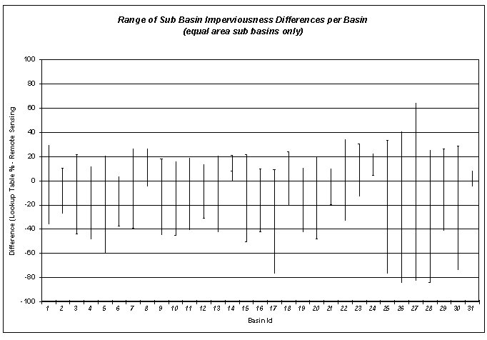
PMR’s remotely-sensed impervious estimates were compared to the KVL impervious values derived through the more traditional lookup tables used in the preparation of the city’s Storm Water Master Plan. Overall results were examined for all 31 major basins. These results appeared inconclusive until basins were analyzed at the sub basin level. Five different basins (1, 7, 8, 25, and 29), reflecting a variety of sizes and conditions, were reviewed in detail.
The original KVL impervious values were based on City land use classifications assigned to parcels of land. The percent impervious values were derived from a national government publication entitled: “Urban Hydrology for Small Watersheds”, U.S. Dept. of Agriculture-Soil Conservation Service TR-55. The land use classifications were converted to average number of dwelling units per acre and the percent impervious value was taken from Table 2-2a in this publication. The table in TR-55 has only one land use category for commercial called “commercial and business” and one for industrial. The other categories are six different residential districts based on average lot size
Some sub basins showed remotely sensed impervious values higher than the lookup table derived figures and others were much lower (Figure 3). Not until the sub basin results were transferred onto a planimetric map of the individual basins, did spatial patterns and consistent results begin to appear. The maps revealed that sub basins with similar PMR values and deviations from the KVL values were spatially clustered.
The results can be classified into one of the following categories:
1) The areas where the results between KVL and PMR values appear most similar are in the older, fully developed residential areas that have a uniform density of number of lots, size of lots, and/or dwelling units per acre. PMR impervious values appear to be consistently slightly higher than the KVL values. This implies the actual impervious areas are slightly higher than the assumed TR-55 values. After a more thorough and detailed analysis of the results, the City will correct the values in its hydrologic model for fully developed areas and adjust the impervious values in the lookup table for use in the remaining undeveloped areas of the city.
2) In other older residential areas larger deviations in the data occurred. This suggests that the city land use classifications used in the KVL study were broad in definition and that the classification system had lumped together a range of land use densities. The PMR remote sensing data actually detected these density differences, which resulted in the greater and inconsistent deviations between the PMR and KVL values. The PMR data more accurately reflect the actual differences in land cover densities, thus explaining why the differences in the PMR values were greater in some areas than in other areas. In fully developed areas the remote sensing data will allow drainage planners to go back and redefine the land use classification boundaries in more detail to reflect actual differences in densities.
3) The commercial areas seem to have the more significant deviations. The KVL impervious area values are consistently higher than the actual PMR remote sensing data. This appears to be the case in some areas because they are not yet fully developed to the maximum extent possible. For areas that appear to be fully developed, a possible alternative explanation is that commercial development within the city may provide more landscaping and open space than the assumed national average; therefore the standard value of 85% imperviousness may be too high. The good news from a planning standpoint is that the assumed conditions for fully developed commercial sites appear to be a desirable safe worst- case condition. Further analysis of the remote sensing data may refine this category into several different classes of commercial and business. In the fully developed commercial areas of the city, planners may be able reduce the estimate of impervious area to reflect the actual conditions determined from the remote sensing data.
The original storm water drainage master planning study evaluated the capacity of existing conveyance facilities and estimated the size and costs for upgrading infrastructure to a 100-year level of protection. Given the higher accuracy of the remotely sensed impervious values, the hydrologic models for each of the five major basins referenced above were re-run with the new data. The results were used to re-consider the construction of proposed conveyance facilities and evaluate their potential fiscal impacts. Basins 7 and 8 appear to have the greatest potential savings.
Basin 7 had only one area with a significant change in runoff. This change permits the reduction of a proposed one-quarter mile long section of 30” diameter storm drain pipe to a 24” diameter pipe. Using the same cost assumptions as the master plan study, this results in a cost savings of $24,700
Basin 8 flows were decreased enough to allow reduction of proposed conveyance facilities at four different concentration points. In one location, 420 feet of a proposed 66” pipe can be downsized to 48” pipe for a savings of $24,200. In another area, three different segments of a proposed 72” pipe can be downsized to 60” over a total length of 1,240 feet. This results in a savings of $48, 300
Based on the re-run hydrology models, it appears that approximately 40% of the sub basin discharge values are within ±10% of the original assumptions, 30% of the sub basins have significant underestimates and the remaining 30% have significant overestimates. This suggests that 60% of the storm water conveyance infrastructure in the study area is improperly sized. While it is too early to determine if these results will result in net dollar savings to the community, it does indicate that planners may be able to target scarce tax dollars more effectively while providing a higher level of protection to residents in the affected areas.
The primary objective of stormwater management in Scottsdale is to minimize the risk of flooding and to protect the health, safety, and welfare of its residents in an efficient, cost-effective manner. This study shows that high-resolution multi-spectral imagery classified with standard techniques and refined with vector data of the type found in many municipalities will allow the City to better meet these objectives in several important ways.
The combination of data and processes used in this project worked well and fulfilled the requirements of the study. The use of remote sensing for determining imperviousness gives municipalities a powerful and cost-effective new tool for stormwater management. Given the potential for major improvements in safety, as well as significant financial savings, assessing the applicability of these techniques in other areas, such as the northern portion of Scottsdale and other dry urban areas, is recommended.
The authors would like to thank the following people for their contribution to this project: Bill Erickson of the City of Scottsdale Transportation Department; and Jennifer Jensen and Carder Hunt of the City of Scottsdale Information Systems Department.
This study was conducted under NASA Grant NCC13-15. The city gratefully acknowledges NASA’s support over the years.
This paper is a modification of one originally presented to NASA under the title "Towards a More Accurate Prediction of Stormwater Run-off: Determining Imperviousness With High-Resolution Remote Sensing Data For Input Into the HEC-1 Model."