
Paul Loechl, Wendy Goetz, Chad Hendrix and Julie Coen
The US Army Corps of Engineers research laboratories has established guidelines for mapping vegetation on army installations to address land management issues on Army military bases. Pacific Meridian Resources has completed one of the first vegetation mapping efforts to follow these guidelines. A vegetation map of the Fort Hood Military Reservation in Killeen Texas was developed using 1-meter scanned digital color infrared Orthophotography Quarter Quads (DOQQ) imagery. A series of unsupervised classification and modeling techniques were used to separate 16 land cover classes. A core component of the project was the development of an ArcView model to eliminate tree shadow areas during classification by utilizing the surrounding vegetation patterns. The integration of GIS modeling approaches with techniques for remotely sensing vegetation classification was a key component to the success of the project. A review of techniques, lessons learned, and issues will be presented.
The development of data about natural resources, such as maps of vegetation communities, is a necessary and important activity at military installations. Trainers need this information to be able to carry out and sustain their mission, and land managers need these data to be able to sustain and protect the installation's land and water resources. These users, and potentially many more, represent many levels of users who need vegetation maps to make decisions important to the installation mission. Each of these users requires that the final map be able to meet their needs for vegetation information, be it concealment patterns and avenues of approach for training simulation, habitat composition and patterns for managed animal and plant species, or as a basic data layer for programs and models designed to assess, manage and sustain the land.
The Army Corps of Engineers developed guidelines for mapping vegetation on Army installations to help installation project managers produce vegetation maps that are economical and useful to a many users. The guidelines, which adhere to Federal Geographic Data Committee's National Vegetation Classification Standard (NVCS), focus on the map development process as a decision framework that must be addressed by the project manager to ensure a successful vegetation map. The framework, described in a document entitled "Guidelines for Mapping Vegetation on Army Installations", was applied as a demonstration/validation study at Fort Hood military reservation in Killeen, Texas. A vegetation map was developed using the Guidelines as a model for five user groups including the training program, threatened and endangered species management, plant succession modeling, carrying capacity modeling, and the soil erosion program.
The usual intent of a vegetation map is to supply an inventory of plant communities including their location, extent, geographical distribution in the landscape, relationship to other landscape features, and a description of selected characteristics. With the growth of computing techniques and advances in remote sensing, modeling, and sampling theory, a vegetation map can now possess a great deal of sophistication. Further, map information is no longer valuable to only a few, but can be shared, manipulated, and presented to serve many clients, each with their own requirements for map detail, resolution, and information. The integration of Geographic Information Systems (GIS) modeling with techniques for remotely sensed vegetation classification played an important role in the success of producing a useful map for Fort Hood. This paper summarizes the GIS techniques and modeling approaches used to produce an installation vegetation map as well as lessons learned.
The Fort Hood Military Reservation (figure 1) is a 217,337-acre training post located in central Texas, approximately 60 miles north of the state capital city of Austin, and 160 miles south of the Dallas/Fort Worth metroplex. Established in 1942, Fort Hood is the largest armored training center in the free world and consists of two divisions. The installation lies on 87,890 ha within Bell and Coryell Counties in central Texas. Fort Hood occupies land within the Crosstimbers and Southern Tallgrass Prairie Ecoregion, near the junction with the Edwards Plateau Ecoregion. The Fort Hood landscape typifies this crossroads of ecological regions. Sixty-five percent of the land area is described as perennial grassland and thirty-one percent as woodland (Unpublished data U.S. Army LCTA program). These lands are used primarily for military training but are managed for multiple use, including recreation, fish and wildlife, and agriculture. Fort Hood also provides breeding habitat for two federally listed neotropical migrants, the black-capped vireo (Vireo atricapillus) and the golden-cheeked warbler (Dendroica chyrsoparia). Nondiscretionary terms and conditions established by the U.S. Fish and Wildlife Service in a Biological Opinion issued in 1993 requires the Department of Army, Fort Hood Military Reservation to establish management plans and conduct scientific studies to minimize potential harm to the listed species. The development of accurate vegetation maps supports programs within these management plans.
Study Area - Fort Hood Figure 1
1. Collection of Background Material
It is important to study reference material and existing information to find out as much as possible about the study area and to find out if there are any relevant efforts, past or present, that support the current vegetation mapping effort. A review was conducted to help understand and appreciate the character of the vegetation, reveal general relationships, disclose affinities to disturbance, and understand the dominant environmental features. This review revealed that a fuel load map had been developed in 1998 using Landsat thematic mapper 30m data. In addition, The Nature Conservancy, which has personnel on post, provided vegetation information that included field plot data collected for monitoring threatened and endangered species. Fort Hood also provided plot data previously collected for land condition and trends analysis purposes. Regional vegetation guides such as from the Audubon Society also were helpful in the initial stages.
Fort Hood supplied all of the ancillary data layers used for the project. The point, line, and polygon data sets were received as Esri shapefiles. The raster digital elevation models were received in ERDAS Imagine and Esri Grid format. The following is a list of all the ancillary data layers received from Fort Hood:
There were two sets of DEMs provided by Fort Hood. The first was a 1-meter DEM produced from radar data. The other was a 10-meter DEM produced from the DOQQs themselves. It was discovered that the 1-meter DEM was detecting variations in individual tree canopies rather than the actual ground elevation. A determination was made that the 10-meter DEM produced from 1999 the DOQQs would be more appropriate to use with the vegetation classification procedures. The DEM was used primarily for producing slope and aspect files.
2. Scoping, Planning and Fort Hood requirements.
Scoping and planning was conducted with Fort Hood personnel to establish their objectives for the map, review background information, and to plan the remainder of the project including mapping parameters such as level of detail, scale, and resolution. As a result, the following requirements were identified:
Requirements defined by Fort Hood
3. Data Acquisition, Interpretation, and Manipulation (Image Classification)
Data Preparation
A total of 36 DOQQs were used in the vegetation classification. The imagery was acquired in February of 1999 and scanned into digital format using a flat bed scanner, rectified, and registered to a UTM coordinate system. The DOQQs were mosaiced together into 4 regions (north, south, east, & west) using ERDAS Imagine 8.3 software. This was necessary due to the large size of the imagery. The boundary coverage of Fort Hood was then buffered by 20 meters and used to clip out the study area regions from the mosaiced DOQQs (figure 2). This process eliminated areas outside the Fort Hood boundary and grouped most DOQQ images with similar characteristics of sun angle or tonal balance. All subsequent work was completed on each individual region.
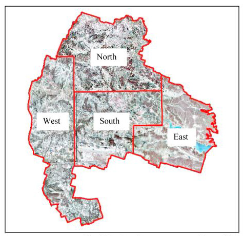
Fort Hood Regions. Figure 2
DOQQ imagery has the following layers:
Band 1 - Blue (represents green)
Band 2 - Green (represents red)
Band 3 - Red (represents the Near Infrared)
The bands do not represent true spectral information because the imagery is scanned from infrared aerial photos. Therefore, no true red or infrared bands exist, only approximations of these bands are available thus making differing vegetation classes difficult to separate. To help identify the vegetation communities a series of ratio bands and indices were developed. Indices combine unique spectral information from two or more spectral bands into a single band that highlights characteristics of interest. Through visual inspection of the resulting images and histograms it was determined that a "pseudo" Normalized Difference Vegetation Index (NDVI) band would provide the best results in combination with the other bands. Research has shown that NDVI bands can be useful in predicting vegetation characteristics. Bands 2 and 3 were used to make a "pseudo" NDVI layer.
IR(band 3) - red(band 2)
IR(band 3) + red(band 2)
This layer was helpful to separate the evergreen tree pixels from the deciduous tree pixels. It was also helpful for differentiating the juniper pixels from Live Oak and for bringing out evergreen vegetation pixels in shadowed areas.
For each region, the "pseudo" NDVI layer was added to the DOQQ imagery as another band. Urban areas were removed from the imagery using an image mask and an 80 cluster unsupervised classification was performed on the non-urban imagery. All unsupervised classifications used an ISODATA algorithm initialized from the image
statistics along a diagonal axis. The convergence thresholds were set to a minimum of 0.96. Each cluster was labeled to one of the following classes:
Water
Bare ground
Grassland/herbaceous
Forest
Shadow
Some initial editing was performed to separate out obvious grass areas that had been confused with the forest clusters. The forest and shadow clusters were used to mask out the imagery again resulting in an image that contained only forest and shadow areas. A 100 cluster unsupervised classification, using the same ISODATA techniques, was run on the forest/shadow imagery and used as an input for CART Analysis.
Field Data Collection
Initially a total of 292 field plots were collected in August of 1999. Field plot locations were selected using a modified stratified random sampling procedure on each DOQQ. The stratification was based on an earlier 1998 Landsat TM based vegetation map. After masking out the developed and restricted range areas, sample site locations were identified based on each of the 1998 vegetation types within each DOQQ. Twenty sample sites were allocated for each DOQQ. The southwest corner of the field plot was manually located to make sure that the plot was a homogenous representation of the appropriate vegetation type. Field plots were gathered by measuring a 20x20 meter square starting at the southwest corner of the field site (figure 3). Plots were not gathered on 11 quads because they were either: located in the impact area or live fire zone, comprised mostly of developed areas, or inaccessible (figure 4).
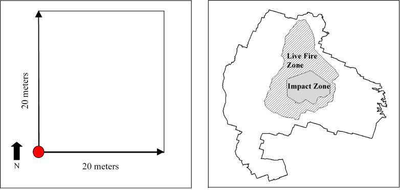
Methodology for gathering field data. Figure 3 Live fire and impact zones. Figure 4
Two levels of field data were collected. The first level included only data on canopy closure, canopy height, percent deciduous, percent evergreen, and the three major tree species of the plot area. The second level included more detailed information on the associated plant species in the plot area. Initially the field data were to be split into two groups: training sites to be used in the classification, and reference data to be used in the accuracy assessment of the final vegetation map. In addition, the field data were also used to develop the descriptions of the vegetation alliances found on Fort Hood.
The data collected in the field were entered into a Microsoft Excel spreadsheet and were statistically analyzed to determine the number of vegetation units present on Fort Hood. The vegetative characteristics of the field plots were analyzed using SAS 6.12 cubic clustering routine. The resulting dendogram and analysis defined 23 vegetation alliances for Fort Hood. The 16 final map classes were latter associated with the 23 vegetation alliances.
An ArcView shapefile of the field plots was generated and then converted to an Arc/Info GIS layer with a unique identification number and vegetation class label for each plot. Each plot was checked for correct placement and site homogeneity. Approximately half of the plots were discarded because of plot misplacement, labeling errors or excessive heterogeneity within the plots.
Eventually it was determined that the field plots could not be used as a training set for the classification of the imagery which is discussed in the CART Analysis section. The plots were too heterogeneous for the resolution of the DOQQ imagery (figure 5). The sites that remained after the quality control check were set aside for accuracy assessment. Due to the number of plots discarded, it was necessary to collect additional field data. Pacific Meridian collected 124 additional plots during one week of field work. Sites were selected using a systematic stratified random sampling technique. This was accomplished by starting in the southwest corner of each DOQQ and assessing the accessibility of that area. If the area was not accessible then the same determination was made on the southeast, northeast, and northwest corners of the DOQQ. At the first area determined to be accessible a 1:1200 scale image plot was made of the area. These image plots were then taken to the field and 5x5 meter homogenous field sites were established for each vegetation class found within the area. These were later entered into a GIS database. An additional 27 water sites were photo interpreted. These plots were manually digitized in using the DOQQ imagery as a reference. Although we attempted to use a portion of the field plots for the initial classification process, it should be noted that none of the original or supplemental field plots were used as training sites in for the final classification process.
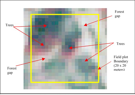
Heterogeniety within field plots. Figure 5
Preliminary Image Classification(CART Analysis)
The field data was intersected with all spectral and ancillary data layers to create a master database. The master database was used as input into a program developed by Pacific Meridian that uses SPLUS 4.5 to generate cluster profile plots and Dbase database files for input into a classification and regression tree (CART) statistical analysis. Both the profiles and CART analysis were tested as aids for model development. Profile plots graphically depict the relationship between the spectral and ancillary data layers and the classes occurring within a particular cluster. One profile was developed for each of the 100 clusters using the master database. Each profile plotted the distribution of the spectral and ancillary data layers. After reviewing the profiles, the database files were used as input into a classification and regression tree (CART) analysis. CART analysis produces dendogram plots and classification rules based on the input data. CART analysis was used to create the first draft classification rules.
After reviewing the results it was discovered there were two problems that deemed CART unsuccessful. The first problem was that the ancillary data layers were driving the CART models. This was basically a result of differences in spatial resolution of the data. The ancillary data layer had a lower spatial resolution than the DOQQ imagery and therefore the ancillary data layers did not contain enough detailed information to make them useful. Ancillary layers are supposed to act as a sieve to filter out the small differences but this was impossible because of the high spatial resolution DOQQ imagery. The second problem was that the 20x20 meter field plots had a great deal of spectral variability which limited or eliminated spectral breaks between different vegetation types. Ideally field plots should be as homogeneous as possible. However, the plots contained other vegetation classes in addition to the target vegetation class causing spectral heterogeneity within the plots. For example, a tree plot not only contained the tree species but contained grassland areas between the canopies, bare ground, as well as other tree species (See figure 5).
Final Image Classification
The decision was made to abandon CART and perform a standard unsupervised classification using statistics to label classes. Using the100 cluster unsupervised classification of the forest/shadow image generated for CART, the clusters were labeled as: juniper, live oak, deciduous, grassland or water. Confused clusters were left unlabeled. Two sets of maps were then made of the unsupervised classification and taken to the field. Regional maps were produced at a scale of 1:10,000 and site specific focus maps were created at a scale of 1:1200. The regional maps were used primarily for navigation and for making notes on the general vegetation composition of an area while focus area maps were used to identify individual trees and clusters on the ground. The maps were checked and used to assist in labeling confused clusters. With the use of the field notes, each of the clusters were given a preliminary label as: deciduous, live oak, juniper, grass, or shadow. Through further modeling process latter in the project the deciduous and grassland classes would be expanded. A shadow class was added to the classification when it was determined that it was impossible to label shadow clusters to one of the other classes without a model. The shadow problems were a result of the spatial resolution of the DOQQ imagery and were intensified by the time of day and time of year the original photos were taken.
A model was developed to eliminate the tree shadow areas by utilizing the surrounding vegetation patterns. Prior to running the model the grassland, bare ground, and water classes from the original 80 cluster unsupervised classification were mosaiced back into the classification. The model was designed to assign values to shadowed areas and areas that were mis-classified due to solar illumination. The model had three phases: first, an orthogonal majority filter was run which removed a minimal amount of noise from the classification. Second, the model assigned the shadow to its respective tree (either juniper of live oak), which became more difficult in areas of dense trees and shadows This phase of the model utilized opposing directional wedge majority filters oriented parallel to the solar azimuth. The final phase utilized a nibble function to eliminate the remaining shadow and replace it with the surrounding vegetation or vegetation that was covered by shadow (figure 6). The results of the model are shown in figure 7.
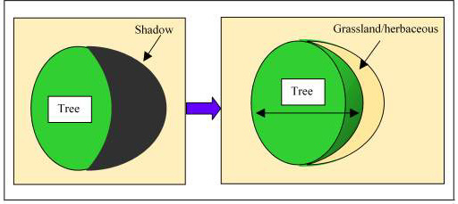
Model uses surrounding vegetation to eliminate shadow. Figure 6
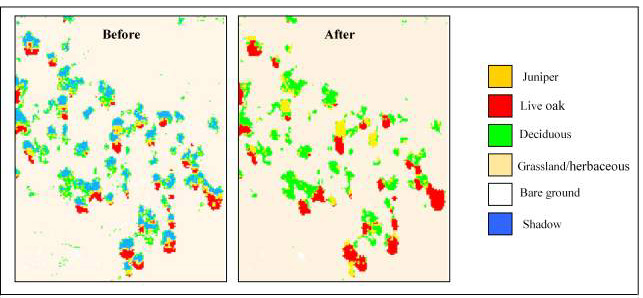
Classification before and after shadow modeling. Figure 7
4. Accuracy Assessment
A total of 299 field plots were used to assess the accuracy of the final vegetation classification. The original 20x20 meter plots were reevaluated and scaled down to 5x5 meters in order to reduce the heterogeneity within the plots. All field plots were now 25 square meters (for a total of 25 pixels). For accuracy assessment the following classes were all called deciduous: maple, north slope deciduous, south slope deciduous, alluvial deciduous, and upland deciduous. The reason for this was that the deciduous classes, except for maple, were based on the 10 meter DEMs and not actual species separation. The accuracy assessment grassland class includes live grassland/herbaceous and dormant grassland/herbaceous. Bare ground plots were not collected.
The error matrix is the standard way of presenting results of an accuracy assessment (Story and Congalton, 1986). It is a square array in which accuracy assessment sites are tallied by both their classified category in the image and their actual category according to the reference data (Lachowski and Maus, 1996). Below is the resulting error matrix for the classes collected at Fort Hood:
Field Plot Reference Data
|
Deciduous |
Grass/ herbaceous |
Juniper |
Live Oak |
Post Oak |
Water |
|
|
Deciduous |
76 |
10 |
4 |
|||
|
Grass/ herbaceous |
6 |
52 |
1 |
5 |
1 |
|
|
Juniper |
4 |
38 |
19 |
|||
|
Live Oak |
4 |
45 |
||||
|
Post Oak |
1 |
1 |
5 |
|||
|
Water |
27 |
|
Vegetation Classes |
Producers Accuracy |
Users Accuracy |
||
|
Deciduous |
76/87 |
87 % |
76/90 |
84 % |
|
Grassland/herbaceous |
52/52 |
100 % |
52/65 |
80 % |
|
Juniper |
38/54 |
65 % |
38/61 |
62 % |
|
Live oak |
45/69 |
80 % |
45/49 |
92 % |
|
Post oak |
5/10 |
50 % |
5/7 |
71 % |
|
Water |
27/27 |
100 % |
7/27 |
100 % |
Overall Accuracy: 243/299 = 81 %
Errors of Omission and Errors of Commission:
|
Vegetation Classes |
Errors of omission |
Errors of commission |
Correct |
|||
|
Deciduous |
11/87 |
13 % |
14/87 |
16 % |
76/87 |
87 % |
|
Grassland/herbaceous |
0/52 |
0 % |
13/52 |
25 % |
52/52 |
100 % |
|
Juniper |
16/54 |
30 % |
23/54 |
43 % |
38/54 |
70% |
|
Live oak |
24/69 |
35 % |
4/69 |
6 % |
45/69 |
67 % |
|
Post oak |
5/10 |
50 % |
2/10 |
20 % |
5/10 |
50% |
|
Water |
0/27 |
0 % |
0/27 |
0 % |
27/27 |
100% |
Discussion of Accuracy Assessment
The overall accuracy of the final map was very good at 81 %. To calculate the individual categories, a producers and users accuracy assessment was done. Producer's accuracy is the percentage of time a vegetation class identified on the ground is classified into the same category on the map. User's accuracy is the percentage of time a vegetation class identified on the map is classified into the same category on the ground (Campbell 1987). The overall user's accuracy was slightly higher than the overall producer's accuracy.
The error matrix also gives you errors of commission (errors of inclusion) and omission (errors of exclusion). Commission errors occur when an area is included into a category when it does not belong to that category. Omission errors occur when an area is excluded from a category when it truly does belong to that category (Congalton and Green 1999). The map showed a high omission error in the post oak category. This means that the post oak class was under represented on the map. The juniper category on the other hand had a high commission error. This means that the juniper class was over represented on the map. The evergreen classes, juniper and live oak, accounted for most of the confusion between map classes.
Other factors that may be influencing the accuracy assessment include; the sample size of the post oak was not large enough to provide a high confidence level in the map class, the maple sites were never sampled due to lack of access, and failing to collect bare ground samples could have effected the overall accuracy as well as the accuracy of the grassland/herbaceous class.
While DOQQ's produced from scanned photos are not the ideal imagery for automated image processing, the resulting classes mapped for Fort Hood have a high level of accuracy. The map portrays the vegetation composition found on the base and the heterogeneous nature of that vegetation. The resolution of the source data provides information not only on the large gaps but also the small gaps found amongst the woody vegetation. The map will prove beneficial in assessing past training effects on wildlife habitat, analyzing the fragmentation of that habitat, and for examining the composition and succession of vegetation communities.
There were many variables that influenced the results of this image classification project. Some of these variables were hurdles that were overcome, others could not be overcome but could be addressed in future projects and coordination between projects. These variables are addressed below.
Scanned DOQQs
1-meter spatial resolution of the imagery
Confusion between the Juniper and Live Oak classes
Leaf-off imagery and Deciduous forests
Campbell, J.B., 1987. Introduction to Remote Sensing, The Guilford Press, pp. 342-348.
Campbell, M.V. et al., 1998. Guidelines for Mapping Vegetation on Army Installations, USAEWES TR EL-98-09, USACERL TR 98/118.
Congalton, R.G. and K.Green, 1999. Assessing the Accuracy of Remotely Sensed Data: Principles and Practices, J.G. Lyon (editor), Lewis Publishers, pp. 45-47.
Lachowki, H. and P.Maul, 1996. Guildelines for the Use of Digitial Imagery for Vegetation Mapping, Engineering Report EM-7140-25, USDA Forest Service, pp. 55-62.
Story, M. and R.G.Congalton, 1986. Accuracy assessment: A users perspective, Photogrammetric Engineering and Remote Sensing, 58(9):1343-1350.
Paul Loechl
Landscape Architect
U.S. Army Corps of Engineers
Engineering Research Development Center - Construction Engineering Research Laboratory
Champaign, Illinois
ph) 217-352-6511 x7443
fax) 217-373-7251
p-loechl@cecer.army.mil
Wendy Goetz
Remote Sensing/GIS Analyst
Pacific Meridian Resources/Space Imaging Services
Salt Lake City, UT
801) 325 1006
801) 325 1009
wgoetz@pacificmeridian.com
Chad Hendrix
Senior Remote Sensing/GIS Analyst
Pacific Meridian Resources/Space Imaging Services
Emeryville, CA
510) 654 6980
510) 654 5774
chendrix@pacificmeridian.com
Julie Coen
Project Manager
Pacific Meridian Resources/Space Imaging Services
Salt Lake City, UT
(801) 325 1006
(801) 325 1009
jcoen@pacificmeridian.com