Lars Brabyn
Department of Geography
University of Waikato
Hamilton, New Zealand
 

Abstract

This paper demonstrates a method for estimating the geographical accessibility of General Practitioners (GPs) using Geographical Information Systems. Cost path analysis is used to determine the minimum travel time and distance to the closest GP via a road network. This analysis is applied to approximately 38,000 census enumeration district centroids in New Zealand and this enables travel time and distance to be linked to the population distribution. Statistics can be generated on what is the average time spent traveling or the average distance traveled if everybody visited a GP once. These statistics can be generated for different management areas and enables comparisons to be made between regions. This accessibility model is intended for decision support for health planners assessing the distribution of GP services. It can also be easily adapted for other services such as access to hospitals and cancer screening centers. A difficulty with calculating travel times is determining the travel speeds for different roads. Road layers often contain information that describes the road characteristics and additional information on the bendiness of the roads can be obtained from calculating the sinuosity of the roads. A process for calculating sinuosity and estimating road travel speeds is described.

Introduction

Accessibility to General Practitioners is a major contentious issue in most countries in the world (Perry and Gesler, 2000) and New Zealand is no exception (Malcolm and Clayton, 1988). Poor access to primary health services, such as GPs, can result in people with simple health problems not being advised by GPs and subsequently developing complex problems with considerable discomfort that can be expensive to treat (Haynes et al, 1999).

Health planners and policy developers require information on accessibility to GPs so that procedures and policies can be developed to address inequities. An important consideration for such decision-making is where people are living and their travel distance and time to the closest GP.

Recent improvements in computer power and the availability of GIS data layers has opened up new opportunities for modeling accessibility. Even though, least-cost path algorithms have been available in commercial GIS since the late 1980s, the application of these algorithms to large national data sets has only recently become feasible. This paper demonstrates how GIS can be used to model travel distance and time to GPs in New Zealand using 1,390 GP Practices (a practice may contain many GPs) and approximately 38,000 population census enumeration district centroids (called meshblocks in New Zealand). This travel is based on using a private car traveling on a road network. The approximate travel time and distance from each meshblock to the closest GP will be calculated. This paper will describe an Arc/Info process to do this, comment on experiences, and demonstrate applications of such a result.

The benefit of having travel time and distance to the closest GP for each meshblock is that by multiplying the travel distance or travel time by the population of each meshblock, it is possible to calculate the approximate total and average travel time and distance if everybody visited a GP once. These statistics can be tabulated for different management areas such as District Health Boards or Territorial Local Authorities and provide a comparison of GP accessibility for different regions of New Zealand. These indices of GP access can be formulated in many different ways so that demographic groups in more need of health care, such as the elderly and the very young, are given extra weighting. These indices can be used to determine the social equity of the distribution of GPs in New Zealand.

Background Information

It should be emphasised that there are many different components to accessibility of health care and geographical accessibility is only one. Other components identified by the World Health Assembly (1979) include financial, cultural and functional. Even, just considering geographical accessibility there are many models that can be used. The use of gravity models and distance decay functions can be used to model spatial interaction and produce indices of accessibility (Fotheringham and O'Kelly 1989). There are also simple density models that show the population per GP for a given unit area.

The use of time and the interrelationship between space and time has an important affect on choice (Huisman and Forer 1998). The shortest path by distance may be totally different to the shortest path by time (Shannon et al, 1973).  Urban areas may appear to have good access to facilities when only road distance is taken into account, but when traffic congestion and low travel speed restrictions are taken into account, accessibility can be very different. Data on travel speeds can be very expensive to obtain, but there are techniques for estimating travel speeds and these are demonstrated later in this paper.

Over the last two decades there have been many studies on geographical access to health. Many of these studies have not based their analysis on a road network and have used Thiessen polygons (Twigg, 1990 and Zwarenstein, 1991). In New Zealand, Critchlow Associates (1995, 1996) undertook two consultancies for the Central Regional Health Authority and the Southern Regional Health Authority that calculated the travel times to public hospitals within each of the commissioning regions. It classified the road network into three speed categories, based on existing Department of Lands and Survey Information road records. Public transport was also incorporated into the database.

Lovett, et. al.'s (2000) study uses GIS techniques to calculate accessibility to a range of primary health services (GPs, pharmacies and dental services) in East Anglia, UK. Separate travel times for both public transport and private car are included. The study used weightings for five different road types that would influence travel speed. It incorporated data on the actual GP that each patient was registered with, rather than assuming that patients would always choose to use the closest medical practitioner.

This paper will demonstrate a geographic model based on cost path analysis to produce layers showing travel time and distance to the closest GP. The advantage of this approach over gravity modelling is that the concepts of the model are easy for decision makers (who may have very little technical understanding) to grasp. Many people, when thinking about accessibility to GPs, would consider how far it is to the closest GP both in terms of distance and time.

Modelling minimum travel distance to the closest GP

Three input layers were used for the analysis; a road network, meshblock centroids, and point locations of the GPs. Fortunately, the NZ Government has recently relinquished its demand for royalties for access to the national 1:50,000 topographic data set, which means that a comprehensive road network of NZ is now available to all researchers. This road network contains various information on road characteristics but does not contain information on travel speed or time for each road segment. To calculate travel distance, road segment length is required and this is easily computed with GIS.

The meshblock centroids were generated from Statistics New Zealand’s Meshblock areas. Meshblocks are the smallest areas used in the distribution of census data and there are approximately 38,000 in the 2001 census release (Statistics New Zealand 2001 – http://www.stats.govt.nz). The unique identification number for each meshblock links these small areas to population census data, which facilitates demographic analysis.

The network analysis capabilities in ARC/INFO were used to calculate accessibility. The key command used was called nodedistance, which computes the distances between all possible combinations of origin and destination nodes. This command uses a least cost path algorithm, which is based on an algorithm generally credited to Dijkstra (1959). The algorithm is described in Arc/Info user manuals (Esri, 1992).  In this study, the nodes closest to the meshblock centroids were the origin nodes and the nodes closest to the GPs were the destination nodes. The nodes closest to the meshblock centroids and GPs were identified using the near command, which also calculates the Euclidian distance to the nodes.

The nodedistance command provides a table of minimum distances via a network between all possible combinations of origins and destinations. It also provides identification numbers of the origins and destinations for each record and the Euclidean distance. The nodedistance function does not only identify distances but can also be used on any specified field, such as travel time. To identify the closest GP for a given meshblock centroid the statistic function in Arcinfo was used to identify the minimum distance for each origin to the closest destination.

The minimum distance to the closest GP for each centroid was calculated by summing the network distance (obtained from the nodedistance command and subsequent statistics) plus the distance from the centroid to the closest road node (obtained from the near command) plus the distance from the GP to the closest road node (also obtained from the near command).

The calculation of minimum travel distance to the closest GP is easy to understand and Arc/Info provides some powerful commands that make this possible. This process produces many output tables and the most difficult part of developing this process was linking all the tables through common identification fields so that the identified closest GPs and their distances can be linked back to the meshblock centroids.

The process for calculating the minimum travel time to the closest GP is similar to the minimum distance process except road travel time was used instead of distance. The difficulty with this process was determining what the travel times were for travelling along the road segments. The method for calculating this is described below. The travel times from meshblock centroids and from GPs to the closest road node were calculated using distance (obtained from the GP-distance modelling process) and a travel speed of 50 km/hour.

The processing time for both travel distance and time was approximately 8 hours using two 750 MHz CPU standard desktop PC computers.

Road network travel times

The estimated road network travel times were based on whether the road was inside or outside an urban area, whether or not it was a motorway, the number of lanes, the surface, and the bendiness (sinuosity).

Urban roads were identified from integrating the road network with a Landcover layer (Thompson 1998). Motorways were identified by using the field "name" and searching for the name "Motorway", and also by manually locating "open speed limit" roads in the Wellington and Auckland urban areas. The number of lanes a road has and the road surface were provided with the road layer.

Sinuosity index have been used in hydrology for describing the meandering of river channels. A simple formula for sinuosity is observed length divided by expected straight-line (direct) length (Haggett and Chorley 1969 p58). GIS easily provides observed lengths of lines.  The straight-line length was calculated for each road segment by creating a new road layer that was a generalization of the original road layer. This generalization involved removing vertices from the road arcs so that there was only one vertex per 500m. This had the effect of straightening the road segments. The lengths of the straightened road segments were then calculated and joined to the original road network using arc Ids. The sinuosity index was calculated by dividing the original length by the straight length. If a road was originally straight, then the sinuosity index will be 1. If a road is bendy then the sinuosity index will be above 1. A very bendy road that turns back on itself (hairpin corners on a hill) may have a high sinuosity score of 4. A sinuosity threshold of more than 1.02 was used to identify bendy roads. This threshold was determined by graphically viewing the sinuosity indices roads in New Zealand and comparing this with the author's personal experience.

The estimated travel speed for each road segment was calculated as follows:
· Sealed urban roads  - average speed: 30km/hr
· Urban motorway- average speed: 80km/hr
· Non urban, 2 lanes, sealed, straight roads- average speed: 80 km/hr
· Non urban, 2 lanes, sealed, bendy roads- average speed: 60 km/hr
· Non urban, 1 lane, sealed, straight roads- average speed: 70 km/hr
· Non urban, 1 lane, sealed, bendy roads- average speed: 40 km/hr
· Metalled straight roads- average speed: 50 km/hr
· Metalled bendy roads- average speed: 30 km/hr

This classification of road speeds is more detailed than that used by Critchlow Associates (1995), which was based on only three classes of roads speed - 80km/h for motorways and high-speed rural roads, 60km/h for slow rural roads, and 35km/h for urban and minor rural roads. The travel time study of GPs in East Anglia (UK) (Lovett et al, 2000) used 12 classes of travel time, but because traffic and road conditions are different in the UK, it is not valid to compare them with NZ roads.

The road segment travel times were calculated from arc lengths and estimated travel speeds.  It needs to be emphasized that the road segment travel times are estimations only. The travel speeds for different road types are not based on scientific empirical evidence but instead on approximations based on personal experience. This process does not take into account urban expressways where average travel speeds could be more than 35km/hr. It also does not consider the effects of traffic congestion and difficult intersection. The network distance and travel times ignore one-way streets.

The travel times of the road network were tested against travel times between major towns published by the New Zealand Automobile Association (AA). The major towns that the AA used were entered into a GIS and cost path analysis generated travel times between each town using the derived road network. Overall the GIS generated travel times was 5.08% less than the AA times. The absolute difference in time, calculated as a percentage of the AA time, was 8.85%. This was considered to be an acceptable difference.

Many meshblock centroids are located on offshore islands or out at sea. These centroids are used to represent people on boats or isolated islands. The distance to the closest GP from these centroids is based on the Euclidian distance to the closest road and the network distance along the road to the closest GP. Sometimes the closest roads to these centroids were roads on islands that did not connect to roads near GPs. This caused a problem that was resolved using two approaches. First road networks on large islands were connected to the main road network by an arc that represented a ferry service route. The travel times for these ferry routes were then estimated from timetable schedules. The second approach was to then delete all roads that were not connected to the main road network in the South or North Islands. The Trace and Nselect commands were used to identify these roads.

Results

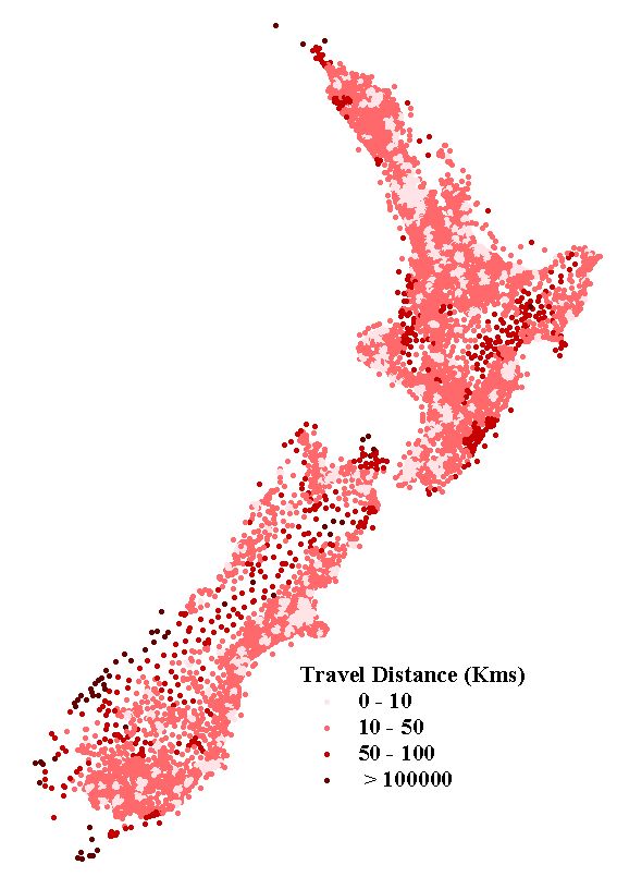
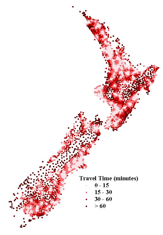
The travel distance and time to the closest GP for each meshblock centroid is represented in Figure 1 and Figure 2. These figures show the raw data that results from the analysis. This data can be aggregated to many different regional management units, such as Territorial Local Authorities or District Health Boards (DHB).

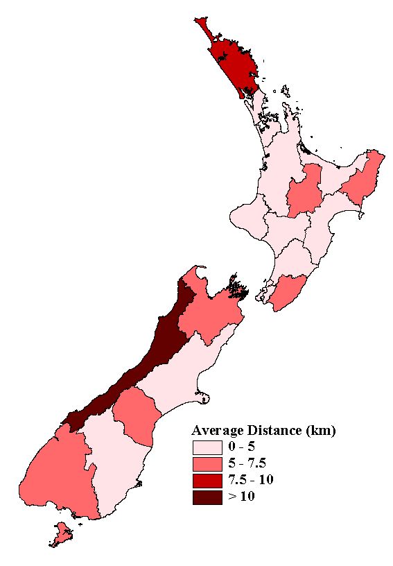
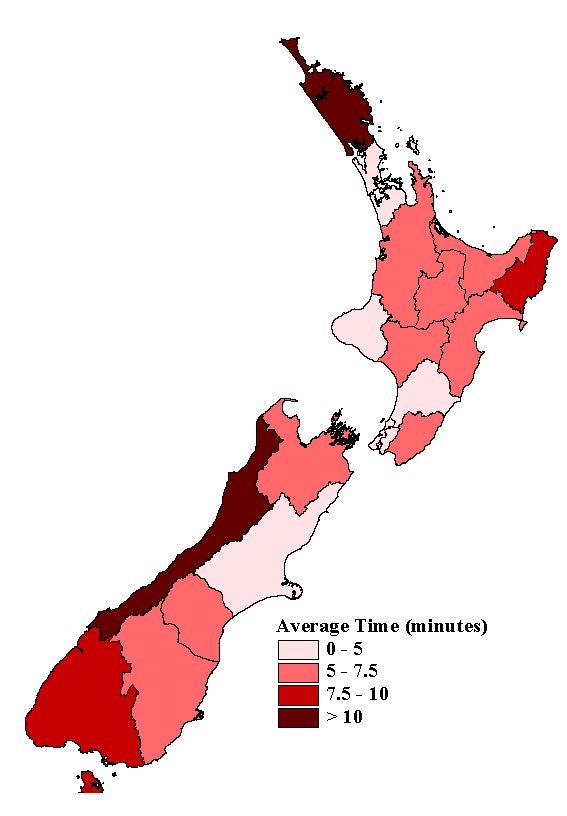
A more meaningful representation of this data would be to also consider the spatial distribution of the population, because there are many areas in New Zealand that have low population densities. Population census data is aggregated to meshblocks therefore it is easy to obtain the population for each meshblock and multiple these by the travel distance or travel time. These products can then be summed for each DHB and then be divided by the population of each DHB to provide the average population distance and the average population time. These averages are shown in Figure 3 and Figure 4.

The "Average Population Time" is the average amount of time spent travelling per person in each DHB if everybody needed to visit the closest GP once. These statistics, based on the population distribution, provide a means of comparing accessibility of different regions throughout New Zealand. The average travel times appear to be very low, especially in some DHBs such as Auckland (1.7 minutes). It needs to be emphasized that these travel times only include actual driving time, not time required to get in the car and finding a car park near the GP. Most people in Auckland would require more time than 1.7 minutes to get to their closest GP because it takes time to load the car (especially if you have children) get the car out the garage, find within vicinity of the GP, and walk into the GP's medical centre. These extra activities could easily add 10 minutes to a journey.

The raw output data produced from the cost path analysis can be applied in many different ways when combined with population data to produce many interesting maps and statistics. However, it is not appropriate to present many maps in this paper. The main intention of this paper is to describe the process used to create the base results, rather than demonstrate applications. It is possible to compare the accessibility of elderly people or different ethnic groups. It can be safely assumed that elderly people need to visit GPs more frequently than other age groups. When calculating total travel times it is possible to put extra weighting on elderly people. Using such weightings and statistics, it would be possible to examine and display the social equity of GP services.

The analysis process not only calculated the distance and time to the closest GP but also identified the name of the closest GP based on both distance and time (sometimes these were different). The number of visits each GP would receive if everybody visited the closest GP once can be easily tabulated and a catchment area for each GP can also be mapped. The average travel speed per GP visit can also be calculated.

Discussion and Conclusion

Geographical access models have enormous potential for informing policy development and grounding debate on how to achieve social equity of primary health care access.  Models are a critical resource that can be used by health service planners to prioritise the location and allocation of health services. The modelling is fairly straightforward and new health services can be processed and existing service access models can be reprocessed quickly on a desktop computer, even for large data sets.

This GIS accessibility model does not take into consideration all factors relevant to assessing access to GP services. Consideration of the availability and cost of public transport is also important because not everyone is able to use a private car. The travel times associated with roads, although based on cost path analysis, also included assumptions that have not been verified empirically, and can therefore only be used as a guide. Further empirical research is required to improve information on road travel speeds. Nevertheless, GIS accessibility models do provide decision support and a relatively consistent method.

When one is developing GIS processes using relatively large data sets and many operations, careful consideration needs to be given to the possibility of error. Logical errors associated with the process and inaccurate data sets can have major effects on the results and considerable caution and cross-checking is required. With powerful computer analysis that is often conducted by one individual, it is imperative that studies be repeated and validated by independent researchers.

The cost path algorithm used in this analysis was based on an algorithm developed several decades ago, but what has changed is the availability of large national databases and computer processing power. This paper has demonstrated that it is now practical to compute accessibility over large networks using thousands of demand points and thousands of supply points. This research has raised the awareness of many public servants of what can be done with GIS, and many are now thinking of other services that should be analysed for accessibility using this approach. With health services alone there are many such services - hospitals, mental health centres, Eye specialists, Oncologists, etc. Health planners are now starting to think of the importance of maintaining geographical databases relating to such services.
 

References

Critchlow Associates Ltd 1995 Access to Health Care and Disability Support Services: Time, Distance, Cost Report - prepared for the Central Regional Health Authority. Wellington

Critchlow Associates Ltd 1996 Access to Health Care and Disability Support Services: Time, Distance, Cost Report - prepared for the Southern Regional Health Authority. Wellington

Dijkstra E W 1959 A Note on Two Problems in Connexion [sic] with Graphs. Numeriske Mathematik, 1

Environmental Systems Research Institute 1992 Network Analysis, ARC/INFO user's guide 6.1. Esri Press.

Fotheringham and O'Kelly 1989 Spatial interaction models: Formulations and applications. Kluwer Academic Publishers.

Haggett P, and Chorley R 1969 Network Analysis in Geography. Edward Arnold, London

Haynes R, Bentham G, Lovett A, and Gale S 1999 Effects of distance to hospitals and GP surgery on hospital inpatient episodes, controlling for needs and provision. Social Science and Medicine 49: 425-433

Huisman O, and Forer P 1998 Computational Agents and Urban Life Spaces: a Preliminary Realisation of the Time-Geography of Student Lifestyles, http://divcom.otago.ac.nz/SIRC/GeoComp/GeoComp98/68/gc_68a.htm

Lovett A, Haynes R, Sunnenberg G, and Gale S 2000 Accessibility of Primary Health Care Services in East Anglia, School of Health Policy and Practice, East Anglia

Malcolm L, and Clayton C 1988 Recent trends in the availability, distribution, utilisationand cost of general practitioner services. New Zealand Medical Journal 101: 818-821

Perry B, and Gesler W 2000 Physical access to primary health care in Andean Bolivia. Social Science and Medicine 50: 1177-1188

Shannon G, Skinner J, and Bashshur R 1973 Time and Distance: The Journey for Medical Care. International Journal of Health Services. Vol. 3, No. 2

Twigg, L. 1990: Health based geographical information systems: Their potential examined in the light of existing data sources. Social Science and Medicine, 30: 1, 143-155

Thompson S 1998 Today's actions tomorrow’s landscapes, Proceedings of the 25 th  Anniversary Conference of the New Zealand Institute of Landscape Architects,  Wellington,  New Zealand.

World Health Assembly 1979 Declaration of Alma-Ata.

Zwarenstein M, Kringe, and Wolff B 1991: The use of a geographical information system for hospital catchment area research in Natal / Kwazulu, South African Medical Journal, 80: 467-500

Acknowledgements

This research has been funded by Public Health Intelligence, which is part of the Ministry of Health, New Zealand. In particular, Dr Chris Skelly has been a key person in establishing the project and suggesting possible goals. Ron King, also from the Ministry of Health, supplied the GP locations and assisted in reviewing the analysis results. I would like to thank these people for there involvement in the project.