Modeling the environment has been one of mans biggest dreams and he has succeeded to quite an extent. When Geographical Information Systems was introduced into the field of environmental management, efforts were made to integrate modeling applications and GIS, so as to facilitate easier management of data and also to create conformity. This paper addresses groundwater modeling which is one of the many entities in environmental modeling. At the time this project was conceived ArcGIS was still in the making and therefore the project was done in ArcView 3.2a. The objective was to create an integrated system where a user could do groundwater modeling in ArcView itself, but the models were run using MODFLOW and MODPATH (USGS groundwater modeling programs) and later do various spatial analyses on the results in the same environment. As is demonstrated in this paper, this objective was achieved for the most part.
Groundwater accounts for about 97 percent of the freshwater resources in the world today (Fetter, 1994). In Illinois, 1453 community water systems (which represent 74% of the community systems in the state) use groundwater as a source of drinking water supply (Illinois Environmental Protection Agency, 1988). Since groundwater aquifers receive recharge from some surficial source, polluting activities by humans on the surface often cause pollutants to reach the aquifer. In fact, a sampling program started in 1985 by the Illinois Environmental Protection Agency (EPA) and the Department of Public Health (DPH), indicated that:
One of the regulatory frameworks available for the protection of groundwater resources in Illinois is the Well Head Protection Area (WHPA). A WHPA, as specified by the Illinois Groundwater Protection Act of 1987, is defined as an area on the land surface from which the aquifer supplying a community with drinking water receives its recharge. The definition of this area is based on a time period, and currently established by the Illinois Environmental Protection Agency (EPA) as five years. However, because the establishment of a WHPA is voluntary and severely restricts polluting activities (which could include agriculture in primarily rural areas), it becomes necessary to determine spatial extent and the economic impact of this measure before communities can adopt it.
A Spatial Decision Support Systems (SDSS), consisting of a GIS and modeling software, could be utilized by rural communities to determine the impact of a WHPA. The goal of an SDSS is to generate alternative solutions to spatial problems, and allow decision-makers to use their judgment to choose from the alternatives. This is necessary because the concept of �bounded rationality� as suggested by Simon (1986) states that humans often make decisions that are limited by their knowledge of the environment. SDSS, therefore, strive to provide the decision maker with a broader spectrum of alternatives to help in the decision making process, usually by incorporating modeling within their framework to answer "what if?" types of questions.
This paper describes the development of an SDSS called ArcMOD that provides decision support capabilities to study the impact of a proposed WHPA on agriculture, and therefore, the economy of largely rural areas. The overall goal is to help communities and Illinois EPA officials make decisions regarding the establishment of WHPAs around groundwater pumping wells that supply communities with drinking water, in accordance with IEPA regulations, in order to protect them from surficial pollution.
Within the SDSS, groundwater modeling coupled with a Geographical Information System (GIS), is used to model and map the creation of a WHPA. Since the groundwater modeling software (MODFLOW) currently has a non-geospatial interface and its own spatial reference system, integrating it with GIS creates a system that allows users to georeference the study area and analyze the results of modeling in relation to other spatial entities (such as cities, rivers, and agricultural areas).
Decision support systems are interactive computer based systems, which help decision-makers utilize data and models to solve unstructured problems (Sprague, 1980). This definition has been further extended over time to include any system that makes some contribution to decision making. The characteristics of DSS are (Sprague, 1980; Densham, 1991):
Spatial Decision Support Systems (SDSS) extend DSS to the spatial level, and support spatial decision-making. The term SDSS refer to computer programs that integrate mathematical models with traditional geoprocessing programs - such as Geographic Information Systems or GIS (Densham, 1991). The models help analyze the data to provide results, which then undergo further analysis in a GIS along with other spatially related data and provide the user with some useful results to help in the decision making process. The SDSS described here integrates the MODFLOW modeling program to determine the spatial extent of a WHPA, and utilizes the GIS overlay function to determine the amount of agricultural land impacted.
Section 1428 of the Federal Safe Drinking Water Act (SDWA) requires each state to submit a wellhead protection program to the United States Environmental Protection Agency. The Illinois Environmental Protection Agency's (EPA) groundwater protection program was approved in 1991, which was also fully complaint with the Illinois Groundwater Protection Act (IGPA) of 1987.
Under this plan, the Illinois EPA created guidelines for the voluntary creation of Well Head Protection Areas (WHPA) by communities dependant on a groundwater pumping well as a primary source of drinking water supply. A WHPA is defined as an area on the land surface from which the aquifer receives recharge over a given time period. This time period, as established by the Illinois EPA, is five years.
Currently, the Illinois EPA is in the process of delineating WHPAs for community water supply wells pumping from aquifers that are susceptible to contamination from the surface. The process of delineation of the WHPA consists of:
MODFLOW is a finite-difference modeling program, which simulates groundwater flow in three dimensions. The code or computer program is written in FORTRAN 77. The program has a modular format, and consists of a �main� program and a series of highly independent subroutines called �modules�. The modules are grouped into �packages�. Each package deals with a specific feature of the hydrologic system which is to be simulated, such as flow of rivers or flow into drains, or with a specific method of solving linear equations which describe the flow system. The division of the program into modules facilitates examination of each hydrologic feature in the model independently. Another advantage of having the modular structure is that new options/features could be added to the program without much change to the existing code.
As with most computer programs that have been available for a long time, MODFLOW underwent several version updates. MODFLOW was originally documented in 1984 by McDonald and Harbaugh (1984). The second version of MODFLOW was documented by McDonald and Harbaugh (1988) and this version is often called MODFLOW-88 to distinguish it from other versions. The third version is called MODFLOW-96 (Harbaugh and McDonald, 1996a and 1996b). The latest version is called MODFLOW-2000 (Harbaugh et.al. 2000). The latest version of MODFLOW, i.e. MODFLOW-2000 has the most number of options/features and thus it was decided that it would be used for the development of the proposed SDSS.
The simultaneous equations used by MODFLOW for each finite difference cell is derived using Darcy�s Law and the law of conservation of mass. The derivation gives a partial differential equation, which is used by MODFLOW. This partial-differential equation of groundwater flow used in MODFLOW is (McDonald and Harbaugh, 1988) is

Where,
Kxx, Kyy, and Kzz are the values of hydraulic conductivity along the x, y and z coordinate axes, which are assumed to be parallel to the major axes of hydraulic conductivity.
h is the potentiometric head
W is the volumetric flux per unit volume representing sources and/or sinks of water, with W<0.0 for flow out of the ground-water system, and W>0.0 for flow in.
Ss is the specific storage of the porous material; and
t is time.
This equation, when combined with boundary and initial conditions, describes transient three-dimensional ground-water flow in a heterogeneous and anisotropic medium, provided that the principal axes of hydraulic conductivity are aligned with the coordinate directions. McDonald and Harbaugh (1988) used a finite difference version of this equation in MODFLOW, where the ground-water flow system is divided into a grid of cells. For each cell there is a single point called node, at which the head is calculated.
The packages that were included in MODFLOW -88 were the basic package, the block-centered flow package, the well package, the recharge package and the solver packages i.e. the slice-successive over relaxation package, the direct solver package and the conjugate gradient package. These packages have been extended in MODFLOW 2000. In addition to the packages mentioned above, MODFLOW now includes the layer-property flow package, the horizontal flow barrier package, the river package, the drain package, the evapotranspiration package, the general-head boundary package, and the constant-head boundary package. (McDonald and Harbaugh, 2000)
MODPATH is a particle tracking program, which computes the paths for imaginary particles of water moving through the simulated groundwater system; it could be said that it is a post-processing program designed to work with MODFLOW (McDonald and Harbaugh, 1988; Pollock, 1994). Particle tracking is a process of tracing out flow paths, or pathlines, by tracking the movement of infinitely small imaginary particles placed in the flow system. MODPATH uses Darcys�s law and the law of conservation of mass in the same fashion as MODFLOW. The results of MODLFOW provide the velocities only at the midpoints of the cell boundaries, if a particle is located inside a cell the velocity is calculated by MODPATH using linear interpolation. In addition to this the average linear velocity and porosity is also used. It has been stated that since the velocity component of the particle at any time are known functions of the particle coordinates, the coordinates of the particle at any future time can also be computed (Pollock, 1994).
The data files that are required by MODPATH (for the implementation of the SDSS with the limited MODFLOW modeling environment) are the name file, main data file, the recharge file, the well file, the time data file, the starting locations file, the flow budget file (generated as output from MODLFOW), the head file (generated as output from MODFLOW). In turn MODPATH generates the endpoint file, the pathline file, and the summary output file as output.
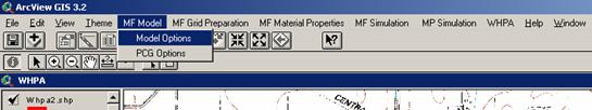
The integrated GIS and groundwater modeling system, called ArcMOD, utilizes a modified version of the ArcView 3.2 interface. The new interface has a new set of menus, tools and buttons that allow the user to manipulate all the required data in a very user-friendly manner. The new set of menu items, namely; MF Model, MF Grid Preparation, MF Properties, MF Simulation, MP Simulation and WHPA (Figure 1) were added to the existing ArcView 3.2 interface. The menu items with MF prefix signify that they are used for MODFLOW, and the MP prefix signifies that they are used for MODPATH. Some custom tools and buttons were also added to the interface. The functionality of the menu items is to guide the user in developing a groundwater model in a simplified fashion and not to burden him with the complex details of the input files.
The necessary input that is required for a groundwater model to delineate a capture zone can be specified as:
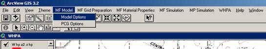
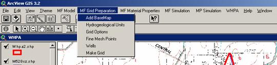
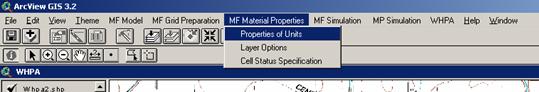
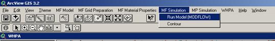
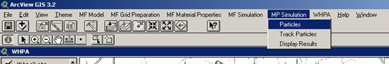
Figure 1: Custom Menus Added to the interface
The menu items guide the user through a process of loading a base map (in the form of an image file) so that the visual-spatial reference is not lost to the user. ArcMOD then provides the user with a tool with which he can specify the boundary of the aquifer as a polygon. The interface takes a zone-based approach at this point, where the user can specify a number of hydrogeological units, each unit having unique aquifer properties (which can be specified and modified at a later stage). The reason for this approach is because in the real world there is often a possibility of modeling an area with two different aquifer units. Specifying the properties of different aquifer is more easily accomplished in the zone-based approach.
There are two types of grids that are most commonly used in making a groundwater model; the uniform grid and the variable grid. The uniform grid consists of evenly spaced rows and columns, thus making all the cells in the grid square. On the other hand the variable grid does not have evenly spaced rows and columns. The reason for variable grids is to provide more detail using a smaller cell size in areas where it is necessary, such as in regions close to pumping wells. Accuracy is also an important consideration when specifying grid dimensions. Since the head distribution consists of heads at the centre of each cell, a smaller the cell-size provides greater accuracy. However, creating uniformly small sized grids for the study area is impractical because it increases computational complexity by providing extra spatial details in area where it is not necessary (e.g., at the boundaries of the aquifer). In a variable grid, this is achieved by having some of the rows and columns spaced close together near areas of interest so that a fine grid that is created by their intersection. The user specifies the minimum cell- size, the maximum cell-size, and the factor by which the cell size should increased when going between the two. Figure 2 shows a grid generated using the automatic grid generation technique.
As stated earlier, the ArcMOD interface takes a zone-based approach. The user is allowed to specify as many units as he wishes. The properties of the zone include top and bottom elevations of the aquifer, the hydraulic conductivity or the transmissivity, the porosity of the aquifer, and the recharge rate of the zone. One limitation is that hydrogeological properties are not allowed to vary within one unit, i.e., the property is constant within a polygon. The dialog box for property input (Figure 3) consists of a pull- down box using which the properties of each of the units can be specified and viewed. The option for interpolation of the properties has been disabled in the dialog box, this being a consideration for future development of the interface. One other input parameter required is the layer option mentioned in earlier during the discussion of MODFLOW. Since the models generated using the interface is limited to single layer models, there is one dialog box (Figure 4) which provides the user with the choice of layer options. Other related inputs that have to specified at this stage include: wells, recharge, and location of particles of pollutant to be tracked.
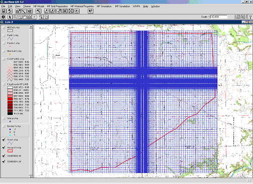
Figure 2: Automatically Generated Grid
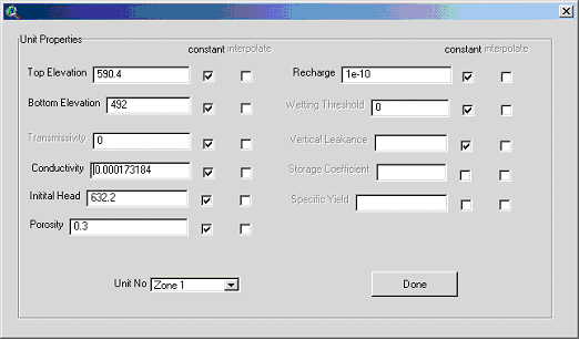
Figure 3: Dialog Box for input of Aquifer Properties
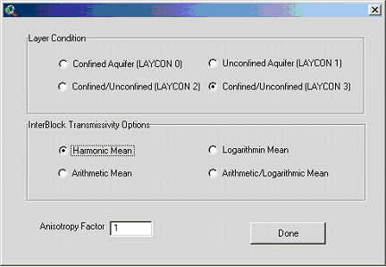
Figure 4: Dialog Box for input of Layer Properties
Well locations can be specified in two ways: by clicking on the screen, or by specifying geographic coordinates. In addition to specifying the location of the well, a discharge rate needs to be specified, i.e., the pumping rate of the well. The dialog box for input of wells is illustrated in Figure 5. Recharge can be specified for each of the zones separately. This is done using the dialog box that allows for input of zone properties. This is assumed to be constant through the zone.
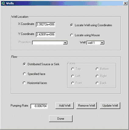
Figure 5: Dialog Box for input of wells
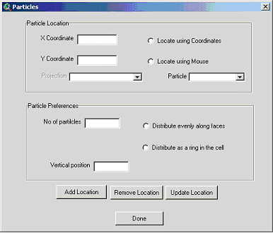
Figure 6: Dialog Box for input of particles
Particles are located in the same way as wells. The input can either be in the form of geographic coordinates or by a mouse click on the screen. The cell (discretized units within the grid) in which the point lies will be the starting location of the particles. In addition to the location of the particles, the user can also specify the number of particles to be located within the cell and how the particles are to be distributed within the cell. There are two options provided for the distribution of the particles in the cell, namely; the ring distribution- where the particles are arranged in the form of a ring with the width of the cells as the diameter of the ring; and even-face distribution, where the particles are located on the boundary of the faces of the cell and evenly spaced along the boundary. The dialog box for input of particles is illustrated in Figure 6. The vertical location of the particles inside the cell can also be specified as factor between one and zero, one signifying that the particle is located at the top of the cell, and zero that the particle is located at the bottom.
After the user has specified the model and has a satisfactory visual model, he can use the ArcMOD interface to call MODFLOW. Avenue uses all the information contained in ArcView at this point to generate the input files for MODFLOW and supplies MODFLOW with the information about the location of the files. MODFLOW then uses these files to run the simulation.
At the request of the user, Avenue accesses the output files generated by MODFLOW. The results from MODFLOW consist of the head distribution in the area modeled. These heads are then associated with each of the respective cells. At this point the interface is back in the GIS environment, and ArcView uses the hydraulic information contained in the cell file output from MODFLOW to generate a contour of the heads. A sample contour from one of the cases simulated is shown in Figure 7.
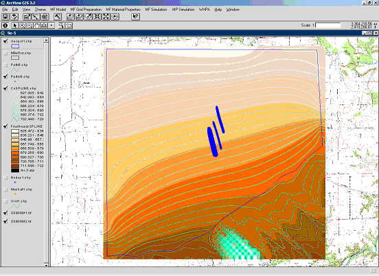
Figure 7: Contour Lines generated for MODFLOW heads output
One of the menu items in the ArcMOD menu contains an item which is the request to generate the WHPA (or the capture zone). The only input at this point is the time for which he wants the particles to be tracked. The default value in the dialogue box is a time period of five years, according to Illinois EPA regulations. Note that the interface is flexible and can handle any time-step or period that the user requires as long as it does not conflict with MODPATH, which is the particle tracking program that Avenue calls. The input files for MODPATH consist of files that were generated as results obtained from the execution of MODFLOW, and additional data. Avenue creates the required input files, and provides this information to MODPATH. Once the execution of MODPATH is completed, Avenue accesses the output file generated in the same fashion as it did for MODFLOW. It then displays the results in two forms: one as points connected by lines (the points representing the position of each particle at the end of each time step), and the second as an enclosing polygon joining the end points of each line.
Since the goal of ArcMOD was to provide Illinois EPA and rural communities with an SDSS that they could utilize to measure the economic impact of establishing a WHPA, the final menu utilizes overlay analysis tools available within ArcView determine the amount of agricultural land with a WHPA. The utility of this analysis is demonstrated with the example of one central Illinois community for which pumping well and hydrogeological data was available to the authors.
The town in question currently uses three wells to obtain its drinking water. The location of the wells and their pumping rate was obtained from the Illinois EPA. These wells obtain water from a Quaternary sand and gravel aquifer.
Additional information required to run MODFLOW, such as hydrostratigraphic units, boundary conditions, as well as acceptable ranges for hydraulic conductivity were obtained from bore-well records of the area, and from pertinent literature. The end members for the range of hydraulic conductivity values were based on field-measurements from areas with geologic materials similar to those found in the study area.
The model grid contains 139 columns and 168 rows with column spacing of 15 meters around the wells, increasing outward towards the boundary of the model. This grid was made using the automatic grid generating option in the interface. A hydraulic gradient matching the regional slope was forced by setting constant head boundaries on the edge of the model that equal the land surface elevation. The contact between the bedrock and surficial deposits was simulated as a no flow boundary, although some exchange of groundwater between these units is possible. Modeling was done under the unconfined/confined option available in MODFLOW (LAYCON 3).
Each cell within the modeled boundaries of the field site required the following input for all simulations (based on data from well logs and topographic maps):
Initial Head � 623.2 feet
Aquifer Top Elevation � 590.4 feet
Aquifer Bottom Elevation � 492 feet
Recharge to the model is not required under the assumption of a constant regional gradient. Hydraulic conductivity measurements from aquifer tests for the region reported a range for hydraulic conductivity from 7.216e-3 to 1.732e-4 feet/second. To determine the sensitivity of the model to the variation in hydraulic conductivity, the model was first run by using the highest value of hydraulic conductivity (7.216e-3 ft/s). Then the hydraulic conductivity was gradually decreased toward until at least one of the model cells went dry. This occurred with a hydraulic conductivity of 3.23e-4 ft/second. Any lower value is unreasonable. Therefore, groundwater conditions that exist within the study area fall somewhere between these two end members. Given this assumption, the model was run for hydraulic conductivity values of 7.216e-3ft/s, 8.8888e-4ft/s, 2.952e-4ft/s, 1.732e-4ft/s. In each run of the model, all the other input factors were kept constant and only the hydraulic conductivity values were changed. For each run of the model a capture zone was developed. The final capture zone was the aggregate sum of all the capture zones, yielding a conservative estimate of the capture zone.
Porosity value required by the model was set to 30%. Sand and gravel deposits can have a porosity ranging from 25-50% (Fetter, 1994; Domenico and Schwartz, 1998; Morris and Johnson, 1967). Numerous studies by the Hydrologic Laboratory of the U.S. Geological Survey show that fine gravel deposits typically have porosity between 25-39% with an average value around 34% (Morris and Johnson, 1967). Rounding down to 30% from the average provides a conservative estimate for defining the capture zone.
Once the model was parameterized, it was executed as a steady-state finite difference groundwater flow model using MODFLOW. This yielded the distribution of hydraulic head in the flow system.
In order to delineate the WHPA, particles were reverse tracked from the three production wells for a period of five years with MODPATH (Pollock, 1989). The trace of the particles approximates the capture zone for these well. A projection of the capture zone onto a horizontal plane defines the WHPA. The next step was to overlay this WHPA over agricultural data. An agricultural landcover map for Illinois was obtained from the National Agricultural Statistical Service (NASS). Called the "Cropland Data Layer for Illinois 1999& 2000", each 30 by 30 meter pixels reflected a specific croptype. NASS created this data by reclassifying the LANDSAT 5 and 7 Thematic Mapper Multi-spectral sensor information. In the final analysis, the amount of agricultural land within a WHPA is calculated using Avenue coding. The results of the analysis include the area of land used for each of the crops. The final results are displayed in the form of table with a landuse/landcover code, the particular type of landuse or crop cover and the acreage of the same. A sample report generated by the interface is shown in Figure 8.
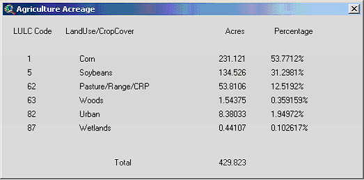
Figure 8: Agricultural Acreage Report Generated by the SDSS
Densham, P.J., 1991, Spatial Decision Support Systems. In D.J. Maguire, M.F. Goodchild, and D.W. Rhind (eds.), Geographical Information Systems: principles and applications, Harlow, Essex, England: Longman,403-412.
Domenico, P.A. and Schwartz, F.W., 1998, Physical and chemical hydrogeology: 2nd Edition: John Wiley and Sons Inc., New York, NY.
Fetter, C.W., 1994, Applied Hydrogeology: Prentice Hall, Englewood Cliffs, NJ.
Harbaugh, A.W. and McDonald, M.G., 1996a, User�s Documentation for MODFLOW-96, an update to the U.S. Geological Survey modular finite-difference groundwater flow model: U.S. Geological Survey Open File Report 96-485.
Harbaugh, A.W. and McDonald, M.G., 1996b, Programmer�s Documentation for MODFLOW-96, an update to the U.S. Geological Surveya modular finite-difference groundwater flow model: U.S. Geological Survey Open File Report 96-486.
Harbaugh, A.W., Banta, E.R., Hill, M.C., and McDonald, M.G., 2000, MODFLOW-2000, The U.S. Geological Survey modular ground water model- User Guide to modularization concepts and the ground-water flow process, U.S Geological Survey open file report 00-92.
Illinois Environmental Protection Agency, 1988, A Primer regarding certain provisions of the Illinois Groundwater Protection Act, IEPA, January 1988.
McDonald, M.G. and Harbaugh, A.W., 1984, A modular three-dimensional finite difference groundwater flow model: US Geological Survey Open File Report, 97-571.
McDonald, M.G., and Harbaugh, A.W., 1988, A modular three-dimensional finite-difference groundwater flow model, Techniques of water resource investigations, 06-A1, USGS.
Morris, D.A. and Johnson, A.I., 1967, Summary of hydrologic and physical properties of rock and soil materials as analyzed by the Hydrologic Laboratory of the U.S. Geological Survey 1948-60: U.S. Geological Survey Water Supply Paper 1839-D.
Simon, H.A., Dantzig, G.B., HOgarth, R., Piott, C.R., Raiffa, H., Schelling, T.C., Shepsle, K.A., Thaier, R., Tversky, A. and Winter, S., 1986, Decision Making and Problem Solving. In: Research Briefing Panel on Decision Making and Problem Solving. Washington D.C. USA: National Academy Press (http://dieoff.org.page163.htm).
Sprague, R.H., 1980, A Framework for the development of Decision Support Systems, Management Information Sciences Quarterly, 4(1), 1-26.
Pollock, D.W., 1989, Documentation of Computer Programs to Compute and Display Pathlines Using Results From the U.S. Geological Survey Modular Three Dimensional Finite-Difference Groundwater Flow Model: U.S. Geological Survey Open File Report 89-381, Denver, CO.
Dr. Raja Sengupta
Professor
Southern Illinois University at Carbondale.
Carbondale IL 62901