Time series analysis of wetland mitigation sites using Spatial Analyst
By Kevin McMaster
22nd Annual Esri International User Conference,
July 11, 2002
Abstract
Land development often necessitates draining or filling jurisdictional wetlands. However, negative environmental impacts are mitigated by construction of new wetlands elsewhere in the same watershed. This paper presents the integrated use of fieldwork, GIS and time series analysis in determining which areas were successfully converted into wetlands for a case-study project. Using an array of 30 monitoring wells, 86 sampling dates, and 1200 spot elevations measurements, all areas that successfully met wetland criteria were identified. A subsequent interactive computer animation helped researchers identify the links between groundwater, precipitation, and variable wetland boundaries.
Introduction
Wetlands filter contaminants, regulate water flow, and provide a natural habitat for plants and animals. Unfortunately land development may require filling or draining natural wetlands. To mitigate the effects of wetland impacts, new wetlands of a similar character may be constructed elsewhere in the same watershed. However, constructed wetlands do not always perform as well as the wetlands they are replacing, and must be monitored to verify an adequate level of mitigation. The U.S. Army Corps of Engineers (USACE) has set the jurisdictional hydrologic success criteria for a wetland as any area that has water within 12 inches of the surface for a continuous 12.5% of the growing season (USACE, 1987). Hydrology must be monitored by ground water well sampling throughout the growing season to confirm the success of the constructed wetland.
Due to the questionable site performance of a previously constructed mitigation site, VHB was asked by the client to assess the site and suggest an improvement strategy (see Fig. 1). GIS played an integral role in this site monitoring, analysis, decision-making, and presentation to the client.
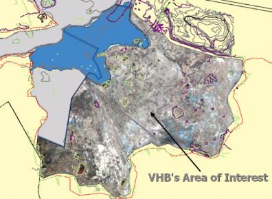
Figure 1. Constructed wetland.
Analysis
Field-surveyed spot elevations from 1200 locations were used to construct a digital terrain model (DTM)
�of the site. ArcView spatial analyst was used to perform in Inverse Distance Weighting interpolation of the spot elevations (see Fig. 2). However the DTM initially did not accurately represent the terrain due to relatively sharp breaks in slope (see Fig. 3).
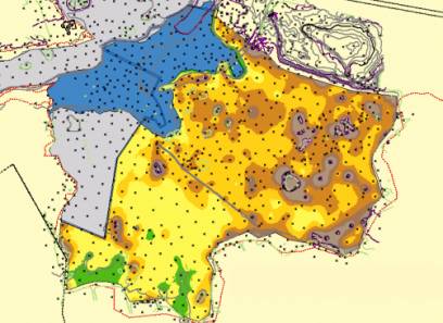
Figure 2. DTM interpolated from spot heights.
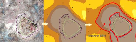
Figure 3. DTM interpolation errors.
To correct for these errors, the spot elevations were used to construct a Triangulated Irregular Network (TIN). Breaklines were identified from the aerial photo and then added as features to the TIN (see Fig 4).
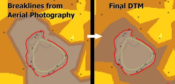
Figure 4. The final DTM using breaklines from aerial photography.
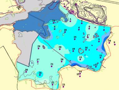
Ground water monitoring wells were installed at 30 locations throughout the site (see Fig. 5). Using data collected weekly, a ground water surface was interpolated using Inverse Distance Weighting and compared to the terrain surface. All areas with water within 12 inches of the surface were reclassified as �saturated areas�, while areas with water above the surface and below 12 inches were reclassified as �surface water� and �unsaturated� respectively (see Fig 6).
 �
�
Figure 5. Monitoring well locations and interpolated groundwater surface.
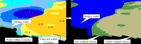
Figure 6. Reclassification based on distance from surface to groundwater.
This analysis was repeated for each sampling date, and the resulting graphics were compiled into an online interactive dynamic model (see Fig. 7). The analytical and visual power of this model has allowed researchers to really see what is occurring throughout the growing season as well as make that information readily available to the client. In addition, the relationship between precipitation and wetland response becomes clear, and measuring the lag-time has allowed researchers to assess dominant contributors to site hydrology (surface water or ground water).
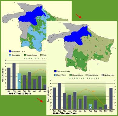
Figure 7. Web-based interactive dynamic model.
To determine which areas were continuously saturated for 12.5% of the growing season (approximately 27 days), the maps were reclassified into binary images based on whether or not they had water within 12 inches of the surface. Keeping in mind that each sample was taken 7 days apart, the following map logic was used:
([Map1] and [Map2] and [Map3] and [Map4]) or ([Map2] and [Map3] and [Map4] and [Map5]) or ([Map3 and etc.) until the samples taken during the growing season were exhausted. The resulting images showed which areas were saturated for a continuous 12.5% of the growing season (see Fig. 8).
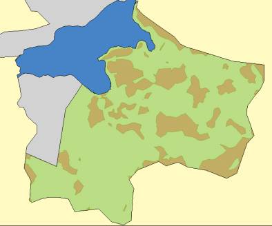
Figure 8. Wetland satisfying the USACE hydrologic criteria.
The wetland map satisfying the USACE hydrologic criteria was used to determined which areas were to be re-graded down a half foot so that they too would meet the jurisdictional criteria for wetlands in the coming years (see Fig. 9).
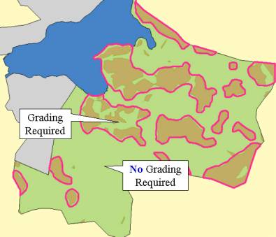
Figure 9. Final map showing areas to be re-graded down 6 inches.
Conclusions
Based on the analytical and visualization capabilities of a GIS, several years worth of monitoring well data were transformed into images clearly showing which areas met the USACE hydrologic criteria for wetlands and which areas did not. By combining model results with field verification, a meaningful conclusion was drawn and remediation actions taken. As a by-product of incorporating GIS into the analytical process, the intermediate images were compiled into an interactive dynamic model that proved to be useful to both environmental analysts, and in presentations to the client. Finally, the lag-times between precipitation and wetland response has allowed researchers to further evaluate dominant hydrologic influences on the site.
References
United States Army Corps of Engineers (USACE). 1987. Corps of Engineers Wetlands Delineation Manual. Wetlands Research Program Technical Report Y-87-1 (on-line edition).
Kevin McMaster, MSc.
GIS Coordinator, VHB Inc.
477 McLaws Circle, Suite 1
Williamsburg, VA 23185
(757) 220-0500
(757) 220-8544 fax
kmcmaster@vhb.com