Ó 2001, Ryan Wilson Smith
DEDICATION
Dedicated in the Memory of my late father, Kent Harley Smith.
ACKNOWLEDGMENTS
I would like to say thanks to Dr. Louis Scuderi, my committee chair, for guiding me through the steps that lead my to my final thesis manuscript.
I would like to thank my committee members, Dr. Seth Snell, and Dr. Kirk Gregory, for their advice and support through the process of writing my thesis.
Thanks to Paul Neville for his advise and help through the beginning processes of developing this classification.
Thanks to all my cohorts that lent help and advice through the process of developing my thesis.
Finally thanks to my wife and son, Shannon and Forrest for their support.
A HYDROLOGIC CLASSIFICATION OF THE EMBUDO WATERSHED, NORTHERN NEW MEXICO
BY
RYAN WILSON SMITH
B.S., Geography, The University of Alabama, 1999
ABSTRACT
This study focuses on the application of using hydrologic parameters in a standard unsupervised classification. This focus is important, because many land classifications fall short when relaying the hydrologic attributes of land cover. Standard land classifications based on spectral response alone look only at land cover as vegetation, not as what areas are most susceptible in producing runoff. This prompts the need for an enhanced hydrologic land classification that incorporates specific hydrologic parameters of elevation, slope, aspect, and texture (surface roughness).
The land cover classification of the Embudo watershed was derived and classified by a K-means unsupervised algorithm. The classification was then improved hydrologically by adding channels of elevation, slope, aspect, and texture (surface roughness). These channels along with the spatial channels of the original classification were classified by a K-means unsupervised classification and evaluated as to their hydrologic parameters. An evaluation of the classes was performed using a GPS survey and field evaluation of the study area.
The hydrologic classes derived in this study should give a better estimate of surface runoff when compared to standard land cover classes derived from spectral bands alone. The final determination of the hydrologic land cover classification compared to that produced by a standard spectrally based land cover classification, will come once incorporated into a hydrologic surface runoff model.
TABLE OF CONTENTS
List of Figures....................................................................................................ix
List of Tables......................................................................................................x
List of Images.....................................................................................................xi
Chapter 1 Introduction.......................................................................................1
Chapter 2 Scientific Background......................................................................6
Chapter 3 Study Area........................................................................................15
Chapter 4 Methodology.....................................................................................17
Chapter 5 Analysis.............................................................................................31
Chapter 6 Interpretation....................................................................................39
Chapter 7 Conclusion........................................................................................42
References..........................................................................................................45
LIST OF FIGURES
Figure1. The Landsat ETM+ platform with multiple attributes of the system shown...................................................................................................................18
Figure 2. A layout created in Arc/View showing GPS points in the watershed and descriptive data assigned to each point...............................................................30
LIST OF TABLES
Table 1. A table of land cover classes derived from an unsupervised K-means classification using Landsat ETM+ bands 1,2,3,4,5,7....................................…..25
Table 2. A table of land cover classes derived from an unsupervised K-means classification using Landsat ETM+ bands 1,2,3,4,5,7, elevation, and slope...….33
Table 3. A table of land cover classes derived from an unsupervised K-means classification using Landsat ETM+ bands 1,2,3,4,5,7, elevation, slope, and aspect...............................................................................................................…35
Table 4. A table of land cover classes derived from an unsupervised K-means classification using Landsat ETM+ bands 1,2,3,4,5,7, and texture (surface roughness)...........................................................................................................36
Table 5. A table of land cover classes derived from an unsupervised K-means classification using Landsat ETM+ bands 1,2,3,4,5,7, elevation, slope, aspect, and texture (surface roughness)..........................................................................37
Table 6. A comparison of the classifications to land cover using Landsat ETM+ bands 1,2,3,4,5,7, and their geographic place in the watershed.........................41
LIST OF IMAGES
Image 1. A Landsat 7 ETM+ scene with band 1-blue, 2-green, 3-red, equalization stretched with a vector overlay of the watershed.................................................16
Image 2. An image of land cover classes derived from an unsupervised K-means classification using Landsat ETM+ bands 1,2,3,4,5,7..........................................24
Image 3. An image with a dissimilarity filter applied to Landsat ETM+ band 2, showing texture (surface roughness)...................................................................26
Image 4. An Image of land cover classes derived from an unsupervised K-means classification using Landsat ETM+ bands 1,2,3,4,5,7, overlain with GPS points.30
Image 5. An image of land cover classes derived from an unsupervised K-means classification using Landsat ETM+ bands 1,2,3,4,5,7, elevation, and slope........33
Image 6. An Image of land cover classes derived from an unsupervised K-means classification using Landsat ETM+ bands 1,2,3,4,5,7, elevation, slope, and aspect..................................................................................................................35
Image 7. An Image of land cover classes derived from an unsupervised K-means classification using Landsat ETM+ bands 1,2,3,4,5,7, and texture (surface roughness)...........................................................................................................36
Image 8. An Image of land cover classes derived from an unsupervised K-means classification using Landsat ETM+ bands 1,2,3,4,5,7, elevation, slope, aspect, and texture (surface roughness)..........................................................................37
Introduction
Land cover is a primary input of hydrologic models for surface runoff. Although it is an important factor, many studies have used land cover classifications that have only marginal information about the surface parameters, which are important hydrologically. Hydrological models whether lumped or distributed require information about landcover. Land cover plays an important role in determining the runoff characteristics of a specific catchment area and can be a determining factor in surface runoff models.
Traditional studies suggest that the type of land cover will affect the type and amount of surface runoff. While these studies are accurate in determining land cover they fall short in determining the hydrologic parameters that can be used in developing a hydrology-based classification. Research on evaluating rural runoff has assumed that there can be a correlation between, land cover and the land attributes that determine soil moisture as well as evapotranspiration rates. It can be asserted that rural land cover classes can contribute to the quantity and delivery rate of storm water and snowmelt runoff to basin water channels. The inability of runoff to infiltrate due to impervious or semi-impervious land covers creates a landscape that produces greater sedimentation and runoff throughout a hydrologic subcatchment. This inability to capture water lends support to the implementation of a hydrologic land cover classification.
This traditional approach towards land classification misses the mark when incorporating useful information about the hydrologic parameters present on the land surface. Many critical parameters such as vegetation type could be more useful when related to percent of vegetation cover, especially when similar species have similar water storage/evapotranspiration characteristics. A hydrologic classification must incorporate the ability to display information not only about vegetative species, but also about the land surface and what classes are important hydrologically. To be useful this classification must incorporate elevation, slope, aspect, surface roughness (texture), and vegetation species derived from satellite imagery and classification of that imagery.
Hydrologic land cover classifications are used to simulate and predict the quantity and/or quality of storm water and snowmelt runoff used in water budgets. Runoff coefficients describe the response of a particular land cover based on surface roughness or texture. It has been shown (ANHIC, 2001) that there is a positive linear relationship between land cover roughness and the amount of runoff that is produced in a given catchment area. As a watershed becomes more impervious or as slope increases, the runoff coefficient characterizing the hydrological response of the watershed can also increase.
Many factors contribute to the potential runoff of a particular land cover; one must study these factors in a hydrological context to produce an accurate classification. The primary hydrologic factors used in this study are vegetative cover, elevation, slope, aspect, and texture (surface roughness). The accuracy of the classification can be increased through the use of a US Geological Survey Digital Elevation Model (DEM) (Wilson, 1997). With the addition of a DEM to increase the accuracy of a classification, one can relate that DEM derived slope and aspect will improve the classification also. These factors should help in the creation of a hydrologic land cover classification that can contribute to the ability of a model to effectively simulate the hydrological response of different land covers and stream flow contributions of a watershed.
There are many theoretical models that describe the use of hydrologic classifications in simulating the hydrologic response of overland flow in a given watershed (Engman and Gurney, 1991). The problem with these models is that few have put the information to good use. When tried they usually fall short for watersheds in the American West. This because the general consensus is that existing land cover classifications are sound, and should be incorporated into a model with no further hydrologic based manipulation.
The definition of the hydrologic parameters required to produce the best possible classification of the land surface can be reached through remote sensing and a Geographic Information System (GIS) analysis of a study area. The use of remotely sensed imagery and coverages GIS provide the means to generate land cover classes that are hydrologic in nature, and which are conducive to hydrologic modeling. One of the greatest objectives of remote sensing is utilizing the data collected by the sensors for the identification and delineation of objects or land cover classes (Kartikeyan, 1994). The promise of remote sensing for hydrologic modeling is tremendous and is slowly being realized in the 21st century (Schultz and Engmann, 2000).
The purpose of this research is to develop and apply a new methodology that produces an accurate hydrologic classification for a small subcatchment of the Rio Grande in New Mexico. This approach combining the classification of remotely sensed data using image processing tools and GIS tools to accurately produce a land cover classification that incorporates digital elevation model (DEM) data. In future research, the classification should be useful for hydrologic models such as the Natural Resource Conservation Service (NRCS data) curve number approach or similar surface runoff model in determining flow rates for the Embudo Watershed.
The land cover classifications and the hydrologic classifications are to be considered final objectives therein to:
1) provide a landcover classification that is hydrological and adaptive to modeling.
2) evaluate the possible effectiveness of the hydrologic classification in predicting surface runoff and stream flow contribution for a given watershed.
3) determine what other data can be used as surrogates in predicting hydrologic responses in the Embudo Watershed.
4) make recommendations for further hydrology classifications or hydrologic inputs.
The Embudo watershed hydrologic classification is a case study that highlights the effectiveness of landcover in determining the hydrological responses of water routing in the Embudo Watershed, Northern New Mexico.
This analysis begins with an unsupervised spectrally-based classification of the study area using Landsat 7 ETM+ bands 1,2,3,4,5, and 7 to determine spectral signatures of the land classes and to delineate the ground area these classes occupy. Next the study explored the possibilities of using elevation, slope, aspect and texture as hydrologic inputs to the classification to better estimate surface runoff. The incorporation of the added digital elevation bands was used to produce a classification that was verified by ground truth data and experts in field analysis. In a final step not taken in this study, the classification should be explored as possible inputs to runoff models and compared to standard land use classifications.
Scientific Background
The process of defining a hydrologic land classification must include background material pertaining to classifications, hydrology classifications, and the models a hydrology classification could accommodate. Land classifications are derived commonly using remotely sensed data. It has its genesis in the development of change detection maps of rural and urban areas in United States during the early 1970's. Land cover is defined as all natural and man made features that cover the earth's immediate material surface (Thompson, 1996). According to Anderson (1976) a land use/land cover classification system which can effectively employ orbital and high altitude remote sensor data should meet the following criteria:
1. The minimum level of interpretation accuracy in the identification of land use and land cover categories from remote sensor data should be at least 85 percent.
2. The accuracy of interpretation for all categories should be about equal.
3. Repeatable or repetitive results should be obtainable from one interpreter to another and from one time of sensing to another.
4. The classification system should be applicable over extensive areas.
5. The categorization should permit vegetation and other types of land cover to be used as surrogates for activity.
6. The classification system should be suitable for use with remote sensor data obtained at different times of the year.
7. Effective use of subcategories that can be obtained from ground surveys or from the use of larger scale or enhanced remote sensor data should be possible.
8. Aggregation of categories must be possible.
9. Comparison with future land use data should be possible.
10. Multiple uses of land should be recognized when possible.
These guidelines are specific to both urban and rural land classifications. Anderson et al, (1976) relates that while there is an obvious need for an urban-oriented land use classification system, there is also a need for a resource-oriented classification system whose primary emphasis would be the remaining 95 percent of the United States land area (Anderson et al, 1971).
Anderson (1976) also states that in the United States Geological Survey (USGS) (www.USGS.gov) classification system the principal points of departure between the USGS system and other classifications originated because of the emphasis placed on remote sensing as the primary data source (Anderson et al, 1976). Because of this emphasis, activity must be interpreted using land cover as the principal surrogate in addition to the image interpreter’s customary references to pattern, geographic location, and so forth (Anderson et al, 1976). The level of detail explained by the USGS method within land cover classifications are sufficient for statewide, interstate, and regional assessments (Anderson level II categorization). Anderson notes that seldom is it necessary to inventory land uses at the more detailed levels, even for local planning (Anderson et al, 1976). In assigning land classification categories it should be emphasized that whatever categories are used at the various classification levels, special attention should be given to providing potential end users of the data with sufficient information so that they may either compile the data into more generalized levels or aggregate more detailed data into existing classes (Anderson et al, 1976).
Thompson (1996) states that in the design of the standard land cover classification the following criteria should be used.
1. The classification should be broad enough to meet the needs of a wide variety of users, and have sufficient flexibility to allow specific user or project requirements to be accommodated, including the use and integration of the additional non-remote-sensing data where applicable or required (i.e. GIS-based modeling).
2. The classification should be based on an a priori hierarchical structure that will allow easy subdivision of broad generic classes into more specific, user or project a posteriori-defined subclasses.
Thompson adds that by using a predetermined classification system (that is, an a priori design), the user and analyst will be able to ensure the final classification structure. The classification (Thompson, 1996) should be based on three hierarchical levels.
1. Land cover types that can be identified using high resolution satellite imagery, such as LANDSAT TM and SPOT, without the use of ancillary data.
2. Subclasses that can be identified from remote sensing data, without the use of ancillary data, if the data format is suitable (i.e. digital, print, scale, season, band combinations, etc.).
3. Flexible, user-defined subcategories developed by individual planners, remote sensing analyst, etc., specific to their own requirements or resource management disciplines.
Thompson (2000) also notes that a structured hierarchical format offers a high degree of flexibility, and has formed the basic structure for several international and national classification systems: for example, the USGS land cover/land use classification system designed by Anderson et al (1976).
The hierarchical data format is a structure that provides the user with the ability to accommodate different levels of information. Therefore broad-level classes represent aggregates of more detailed subclasses, or of new aggregate classes (Thompson, 1996). Such a classification is designed to simplify information so that it can be used by a variety of users with multiple skill levels.
Final land cover classes should be appropriate to both the user's requirements and the objectives of the mapping exercise, and they must be based on cover types that can be reasonably interpreted from satellite imagery (Thompson, 1996). Both Anderson and Thompson explain that any classification scheme should be flexible and should be derived from satellite imagery where vegetation types in a study area can be visibly interpreted to real classes and names assigned to real world land cover groups.
Gregorio and Jansen define land cover as the observed physical cover including the vegetation (natural or planted) and human constructions which cover the earth's surface (Gregorio and Jansen, 1996). According to them, land cover classes are defined by the combination of a set of independent diagnostic criteria, the so called classifiers, which are hierarchically arranged to assure a high degree of geographical analysis (Gregorio and Jansen, 1996). A classification allows the use of the most appropriate classifiers and reduces the total number of impractical combinations of classifiers (Gregorio and Jansen, 1996).
The results of a classification obtained from satellite images by conventional methods can be improved if the spatial information is considered jointly with the spectral information in the same strategy of classification (Swain et al, 1979). Alonso and Soria relate that the spatial information contained in the satellite images can be subdivided into two types: texture and context (Alonso and Soria, 1988). Texture refers to a description of the spatial variability of tones within part of a scene (Gurney and Townshend, 1983). Vegetation structure is also a determinant of surface roughness that models require for energy and momentum transfer (IGBP-DIS LCWG, 1995). When using surface roughness or texture it is intuitive in a classification to hypothesize that the ground cover type of a given pixel is not independent of the ground cover types of its neighboring pixels (Alonso and Soria, 1988).
There is limited information available regarding the actual implementation of a hydrologic based land classification and most are theoretical in nature (Engman and Gurney, 1991). Suggesting parameters that can be incorporated into a hydrologic classification. Researches and people who use hydrologic models would like to see the incorporation of remote sensing derived data which would provide precise information about snow hydrology, evapotranspiration, runoff, soil moisture, groundwater, and water quality.
For this study I explored the literature pertaining to estimates of runoff specifically pertaining to and better ways that remote sensing can be incorporated in detecting surface runoff. Engman and Gurney (1991) state that there are two areas where remote sensing contribute to computing runoff specifically:
1. remote sensing used to produce input data for a class of empirical flood peak, annual runoff, or low-flow equations, and,
2. runoff models that are based on a land use component that has been modified to use digital analysis or image interpretation of multispectral data to delineate land cover classes.
Land cover is an important characteristic of the runoff process that affects infiltration, erosion, and evapotranspiration (Engman and Gurney, 1991). Thus, almost any physically based hydrologic model uses some form of land cover data or parameters based on these data (Engman and Gurney, 1991). It should be kept in mind that remotely sensed data are not only used for monitoring of hydrologic state variables, but also as the basis for parameter estimation of hydrologic models (Schultz and Engmann, 2000). Most recent work on adaptive remote sensing to hydrologic modeling has been with the NRCS runoff curve number model (US Department of Agriculture, 1972). The NRCS land cover based runoff equation is:
Q = (P - Ia)2 / (P- Ia) + S
1. Where Q equals runoff.
2. P is volume of rainfall.
3. Ia is the initial abstraction of land cover parameters.
4. S is a retention parameter.
S is defined as the sum of Ia and the potential maximum retention of the watershed. Conceptually Ia represents the interception, infiltration, and depression storage that must be satisfied before runoff begins (Engman and Gurney, 1991). A general consensus is that remotely sensed data will be extremely valuable, but current techniques must be modified or new procedures developed to use these new data forms optimally (Engman and Gurney, 1991).
The last step in producing a hydrologic classification is to look at the applications of modeling such a classification. With no model to test the hydrology classification the classification would be purposeless. Runoff cannot be directly measured by remote sensing techniques (U.S. National Report to IUGG,1995), however, there are two general areas where remote sensing can be used in hydrologic and runoff modeling:
1. Determining watershed geometry, drainage network, and other map-type information for distributed hydrologic models and for empirical flood peak, annual runoff or low flow equations, and,
2. Providing input data such as soil moisture or delineated land cover classes that are used to define runoff coefficients (U.S. National Report to IUGG, 1995).
Of these areas it is important to note that topography is a basic need for hydrologic analysis and modeling (U.S. National Report to IUGG,1995).
When choosing a model the user must think of the particular application the model will be placed. The model chosen for a particular application must balance the scale of the watershed and the appropriate process representation with the model data requirements and data availability (Kite and Kouwen, 1992). One example is that a lumped hydrologic model can be improved by computing the rainfall-runoff and snowmelt processes separately for different land cover classes (Kite and Kouwen, 1992). It has been shown that even random land cover classes within a watershed boundary can possibly determine the hydrological parameters of each unique landcover class within a mountainous watershed (Kite and Kouwen, 1992).
Traditionally, hydrologists have sought to apply rainfall runoff and snowmelt models to hydrologically homogeneous area, typically sub-basins (Kite and Kouwen, 1992). In real life these homogeneous watersheds are impractical and very hard to delineate. For modeling purposes the location of land cover within a computational element may not be as important as the relative amount of each cover (Kite and Kouwen, 1992). In a model the number of land classes that can be practically considered depends on two factors:
1. The number of hydrologically significant classes that can be identified by remote sensing and/or other means, and,
2. The number of stream-flow gauges that are available for optimizing the parameters (Kite and Kouwen, 1992).
Kite and Kouwen suggest that the number of stream gauges should equal or exceed the number of landcover classes being considered. They also suggest that the SLURP (Kite G.W., 1978) model would work nicely in determining a hydrologic output compared to more complex hydrologic models. It is my view that a hydrologic based classification would compliment this model in determining surface processes.
Kouwen et al, (1993) states that most models in current use are lumped conceptual models that use basin averages for meteorological inputs and watershed characteristics. They suggest that a distributed model approach would incorporate the spatial variability of watershed land cover and meteorological processes and therefore should be far less prone to the calibration and extrapolation problems of their lumped predecessors (Kouwen et al, 1993). Spatial variability in basin characteristics in most distributed models is captured using small sub-basin elements called hydrologic response units (HRU's) (Leavesley and Stannard, 1990). With future developments in models and the speed at which sensors are improving it is likely that there will be greater need for hydrological classifications in further research. Remote sensing can provide much of the necessary data to supplement conventional data to expand hydrology in new directions and also provide entirely new data types and forms that will help hydrologist tackle previously unsolvable questions (U.S. National Report to IUGG, 1995).
Study Area
The Embudo watershed is located in north central New Mexico just south of the town of Taos, New Mexico. The main towns located within the watershed are Penasco, Vadito, and Dixon, New Mexico; all of which have small populations and which have economies based on agriculture. The basin is small in size with an approximate area of 516 square kilometers, and an approximate perimeter of 136 kilometers. The bounding coordinates of the subset study area are upper left 412,155.00 east, 4,022,625.00 north, and lower right 473,565.00 east, 3,976,875.00 north, using Universal Transverse Mercator (UTM) zone 13 WGS84 ellipsoid. The subset can be seen in Image 1, which uses ETM+ band 1 as blue, band 2 as green, and band 3 as red all stretched with an equalization enhancement; included is a vector overlay of the watershed. The basin has the Sangre de Cristo Mountains bounding its eastern boundary and the Rio Grande valley bounding its western boundary. The highest peak in the watershed is Trampas peak standing approximately 3689 meters (12175 feet) above sea level. The lowest point in the watershed is located at the confluence of the Embudo creek and the Rio Grande standing approximately 1794 meters (5920 feet) above sea level. The watershed is sparsely populated and has very few major roads leading from location to location.
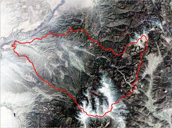 |
Image 1
Methodology
The first part of designing a hydrologic-based classification is to find data that can be used to determine the parameters of land cover within any given study area. For this study the first objective was to find an image that had no visible cloud cover or atmospheric interference for the catchment area. I picked a clear image of northern New Mexico that was acquired during the first week of May 2000 by the Landsat 7 ETM+ platform. The ETM+ instrument on the Landsat 7 spacecraft contains sensors to detect earth scene radiation in three specific bands (NASA, 2001):
1. Visible and near infrared (VNIR) bands - bands 1,2,3,4,and 8 (PAN) with a
spectral range between 0.4 and 1.0 micrometers.
2. Short wavelength infrared (SWIR) bands - bands 5 and 7 with a spectral range
between 1.0 and 3.0 micrometers.
3. Thermal long wavelength infrared (LWIR) band - band 6 with a spectral range
between 8.0 and 12.0 micrometers.
The Orbital Characteristics of the Landsat 7 ETM+ platform are listed below and identified on Figure 1 (NASA, 2001):
· Altitude: 705 km
· Inclination: sun-synchronous, 98.2 degrees
· Descending Node: 10:00 a.m. (+/- 15 minute equatorial crossing time)
· Repeat cycle: 16 days, 233 orbits/cycle
· Period: 98.884 minutes
· Argument of Perigee: 90 degrees (+/- 40 degrees)
Once the image was obtained and bands split into reflective/infrared bands 1,2,3,4,5,7, thermal bands 6l, 6h, and panchromatic band 8 images the next logical step was to geocorrect the image to real world coordinates for proper overlay of a delineated watershed.
Geocorrection can be accomplished by using global positioning system (GPS) points as ground control points (GCP's) or by using an image to image registration using GCP’s of know locations present on both images.
 |
Figure 1
The image after verifying location and accuracy, was then overlain with a geocorrected watershed coverage to ensure the accuracy of the assessment of visible land features. The Rio Grande, Embudo Creek, and two peaks on the eastern edge of the watershed, all, which are visible on the image and on the grid, were used for this assessment. The watershed that is used for accuracy assessment and comparison was derived in Arc/Info from a USGS digital elevation models that had been mosaiced and converted to grid form.
Standard GIS based delineation of the watershed was derived from the surface hydrologic analysis in Arc/Info grid (Esri, 1994). The 30-meter DEM’s were first downloaded from the USGS web site (USGS, 2000) and mosiaced together in Arc/View using the mosaic grid extension. Next the mosaiced DEM was brought into Arc/Info (v 8.0.2) for further analysis in Arc/Grid.
In deriving the watershed from the mosaiced grid I followed the procedure outlined below. First I determine the focal mean so that sinks and depressions prevalent in the grid could be filled. Next I computed flow direction so that the steepest descent is specified from one of the neighboring eight cells adjacent to the principal flow cell, from this a flow direction grid was derived. A flow accumulation routine in Arc/Info Grid was then used to specify which cells would receive the most water as surface runoff occurred, and which cells would most likely be defined as stream channels. Once flow accumulation was computed the stream network was defined using the number of contributing cells to the stream channel. For this study an iteration of cells contributing with more than 5000 cells flowing into them and an iteration of cells contributing with more than 10000 cells flowing into them were assigned the number 1 and used in determining the stream channel network, all other cells were labeled no data. The stream was then linked and confluence’s identified so that even flow across the watershed could occur. The last steps involved in the grid procedure was to:
1. Delineation of the watershed from the flow direction and linked network grids.
2. Specification of a pour point from which to draw the watershed boundary.
For this study the pour point for the Embudo watershed is located at 417,501.17 east and 4,007,957.83 north, (UTM, NAD 83 projection). Once this was accomplished further extraction of data for the hydrologic classification of the land surface could begin.
After determining that the image and the watershed was overlain properly I made a subset of the image using algorithms in PCI-Works to get a better match of the study area to its true boundaries. The subset was run twice so that the image size matched closely to the study area and a watershed boundary created in Arc/View. To better visualize the pixel values of the image I ran an equalization stretch using the raw values to match the eight-bit scale of the image.
Next I created vector shape files that would be imported into PCI to determine the exact location of the stream network. I used ArcView and converted the watershed and stream network grids into vector coverages, which were saved as Arc/View shape files. I then took the original grid derived from the USGS DEM and the computed slope and aspect grids from it. This coverage was then clipped the stream flow accumulation shapefile to that of the watershed and visually compared a geo-tiff of the image that was exported from PCI. The derived grids matched the geo-tiff of the image to within acceptable tolerances for the classifications, however the DEM, slope, and aspect grids needed to be clipped to match the watershed for further analysis. This was achieved by reclassifying the watershed grid using map algebra so that everything inside the watershed would be multiplied by the value one and everything outside the watershed would be multiplied by the value zero. Once the mathematical reclassification was performed the map calculator in ArcView was used to multiply the, DEM, slope, aspect, and stream network grids and to clip them to the watershed.
With the watershed defined and the accuracy of location verified by physical land features, I used the PCI software to perform unsupervised classifications on the image. For the first classification I used a subset of the reflective/infrared bands 1,2,3,4,5, and 7 assigning them as channels 1,2,3,4,5,6. I ran a k-means unsupervised classification for bands 1,2,3,4,5, using channel 6 as the output channel for the classification. Next I used the same bands and channels, but ran the unsupervised for bands 1,2,3,4,6, using channel 5 as the output channel for the classification. These iterations were done to compare the differences of using visible bands and samples of Infrared bands as different output channels.
The classifications both consisted of eight classes that were displayed using a random pseudo color table. Once this was done I added an extra 8 bit channel and ran the classification using all reflective/infrared bands 1,2,3,4,5,6 and output the results to the new channel 7 consisting of eight unsupervised classes. Eight classes were chosen when compared to other images that were run using more than eight classes. The eight unsupervised classes were chosen due to the homogeneity of land cover in the study area and the need for no further detail beyond that provided by the eight classes.
After the unsupervised classification I verified the results by comparing them to other land use/land cover classes from the USGS. I exported the land use/land cover, soils, geology, and gap vegetation interchange files from the New Mexico Resource Geographic Information System (RGIS) data set by Earth Data Analysis Center (EDAC, 1998). Once the interchange files had been exported into coverages within Arc/Info I was able to display the coverages in ArcView for further analysis.
In ArcView the projections of the land use/land cover and gap vegetation quads were checked for their projection and coordinate X,Y pairs. The projections were verified and the adjacent quads were merged into one covering the study area and the immediate adjoining area of the quads, these were then exported as ArcView shapefiles for further analysis. The procedure was repeated for the soils and geology quads of the study area.
Once the shapefiles were created they were clipped to the watershed as vector shapefiles consisting of data within the Embudo watershed study area. The land cover was then labeled according to Anderson classification level II categories and polygons dissolved accordingly. From these shape files maps were printed to help assign visual representations of a later unsupervised classification by K-means to be conducted of the study area within PCI. There are several variants of K-means clustering algorithm, but most variants involve an iterative scheme that operates over a fixed number of clusters, while attempting to satisfy the following properties:
1. Each class has a center, which is the mean position of all the samples in that class.
2. Each sample is in the class whose center it is closest.
(Overview of K-means clustering, 2001)
Then in ArcView I exported the clipped Embudo DEM and converted it to an ASCII grid that would be imported into PCI. Using PCI image processing software I assigned the unsupervised classification categories by using the landuse/landcover Anderson class II polygon categories and the gap vegetation that were clipped to the watershed, as well as expert and personal knowledge of the study area. For the first classified image with bands 1,2,3,4,5 reflective/infrared classed by K-means I assigned:
1. Evergreen Forest Land
2. Mixed Forest Land
3. Shrub and Brush Rangeland
4. Cropland and Pasture
5. Barren Land
6. Shrub and Brush Tundra
7. Bare Exposed Rock
8. Mixed Tundra
For the second image using bands 1,2,3,4, and 6 reflective/infrared and for the third image using all bands 1,2,3,4,5,and 7, I classed by K-means and assigned the same set of classes.
These two approaches were very similar in classification and showed the same spectral response for the prevalent land surfaces. These spectral responses can be seen on Image 2 and the classes assigned in Table 1.
In PCI the ASCII grid was added as a channel to the classified images. The header of the grid was changed to fit that of the image, using the row and column numbers in the image header while still retaining the 30-meter spatial grid resolution. The objective now was to classify the reflective/infrared channels with that of the DEM derived information, namely elevation, slope, and aspect. The problem that faced the hydrology classification was that the data was scaled in
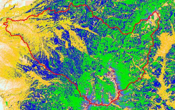 |
Image 2
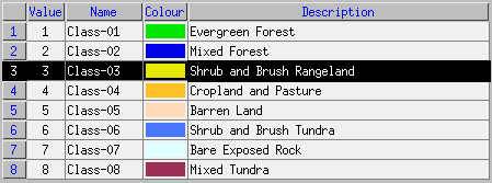 |
Table 1
two categories, the reflective/infrared bands of the image were 8 bit unsigned while the DEM derived data were 16 bit signed. For this problem the DEM data was re-scaled linearly from 16 bit signed to 8 bit unsigned using numerical bounds of elevation, slope, and aspect data. Once this was accomplished a hydrology based unsupervised classification using reflective/infrared bands 1,2,3,4,5,7 and DEM derived bands of elevation, slope, and aspect was accomplished. At this time since aspect played a major role I excluded it and ran a classification of reflective/infrared bands 1,2,3,4,5,7 and DEM derived bands of elevation and slope for contrast. This showed a much different image than the one with aspect included, showing that aspect is very influential in the hydrologic classification.
Next I incorporated texture into the classification by using the dissimilarity filter algorithm in PCI with a 51 by 51 pixel sized filter as seen in Image 3. Vegetation structure is a determinate of the surface roughness length parameters that many models require for energy and momentum transfer equations (IGBP-DIS LCWG, 1995).
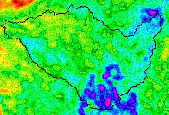 |
Image 3
Edge effects during the texture process were removed during classification by a bitmap image mask classifying only the area of the watershed. The texture algorithm was assigned a channel that was 32 bit real and had to be re-scaled to a linear 8 bit unsigned channel for classification purposes. Once this was done a hydrologic classification using reflective/infrared bands 1,2,3,4,5,7, plus DEM derived bands of elevation, slope, and aspect, and the band assigned texture was performed. At this time an additional iteration using bands 1,2,3,4,5,7 with the added texture band was processed into eight unsupervised classes to see the results of just vegetative cover and texture. The final iterations produced a total of five unsupervised classifications, four of which are important hydrologically and need further study as inputs to hydrologic models.
The last step in validating the classifications was to field verify the Embudo watershed classes using GPS positioning, and confirmation of vegetation types compared to the unsupervised classifications. To do this I used a Trimble Geoexplorer III global positioning unit (GPS) to verify vegetation types in the watershed. For areas that were not accessible due to snow experts verified my classification results. The points collected were used to characterize the classification and were taken and labeled according to the prevalent vegetation surrounding the exact GPS position. These hydrologic classes are:
1. Evergreen Forest Land
Containing species of Ponderosa Pine, Alligator Juniper, Engelmann Spruce, and Douglas Fir. Hydrologically exhibiting 80% canopy cover or more with a low runoff potential.
2. Mixed Forest Land
Containing species of conifers listed above along with mixed deciduous, and some tall shrub and brush vegetation. Hydrologically exhibiting 70% canopy cover or more with a low to moderate runoff potential.
3. Shrub and Brush Rangeland
Containing species of arid shrub and brush vegetation along with small Pinion and Juniper (woody stem) species. Hydrologically exhibiting 30% to 70% canopy cover with a moderate to high runoff potential.
4. Cropland and Pasture
Containing species of high altitude agriculture. For the time of the year of this GPS confirmation idle cropland was prevalent. Hydrologically exhibiting no canopy cover with high runoff potential.
5. Barren Land
Containing no species except for occasional shrub and brush type. Hydrologically exhibiting less than 10% canopy cover with high runoff potential.
6. Shrub and Brush Tundra
Containing species of high altitude shrub, brush and grass vegetation. Hydrologically exhibiting 60% or greater canopy cover with moderate runoff potential
7. Bare Exposed Rock
Containing bare exposed rock outcroppings with no vegetation. Hydrologically exhibiting no canopy cover with high runoff potential.
8. Mixed Tundra
Containing sporadic species of high altitude woody stemmed, berry plants, grasses, and other tundra vegetation with mixed barren ground. Hydrologically exhibiting less than 40% canopy cover with moderate to high runoff potential.
The GPS unit recorded points in UTM NAD83 projection and stored attributes to a generic data dictionary describing the type of prevalent vegetation, estimated percentage of canopy cover, and soil erosion potential due to surface runoff. These points and attributes were then downloaded through the Pathfinder Office GPS software (Trimble, 2001) and saved as an Arc/View shape file. Pathfinder GPS data was also saved from the local base station located at New Mexico Engineering and Research Institute (NMERI) in Albuquerque New Mexico. The shape files were brought into Arc/View and verified as to their location and vegetation type present on a geo-tiff and the DEM of the watershed as seen in Layout 1. At this time the points were also brought into PCI as a vector layer and vegetation type confirmed by comparison to the unsupervised classifications and directly compared to the original land cover classification as seen in Image 4. The vegetation types present on both data sets showed the classification was accurate and the prediction of surface runoff potential could be extrapolated within a model.
Description of statements made in figure 2 are listed below.
pj = pinion/juniper, br = barren, shrb = shrub, rof = runoff, clsd = closed (canopy),
mxed = mixed, cnfr = conifer, cvr = cover, can = canopy.mxed = mixed, cnfr = conifer, cvr = cover, can = canopy.
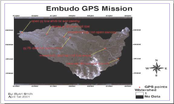 |
Figure2
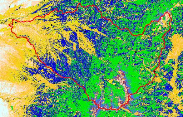 |
Image 4
Analysis
During the course of analysis there were many iterations of vegetative land cover classifications. Classifications using the reflective/infrared bands were all very similar in their vegetative groupings. Images show that the vegetative classes are similar for species across the study area for all classifications, except where there are human derived agriculture plots, strip mines, and physical locations of that nature. These areas changed slightly from one set of bands to another used in the unsupervised classifications. The results of each vegetative land cover classification produced much of the same classes that are described below. These classes are listed below and seen in Table 1:
1. Evergreen Forest
2. Mixed Forrest
3. Shrub and Brush Rangeland
4. Cropland and Pasture
5. Barren Land
6. Shrub and Brush Tundra
7. Bare Exposed Rock
8. Mixed Tundra
These classes were verified by initial comparison to gap vegetation, USGS land use/land cover, expert verification, and personal knowledge of the study area (later verified by GPS, and expert verification).
Once the classes were established for vegetation cover, the DEM derived layers were added and unsupervised classifications run again for the study area. These new classes showed the relevance of elevation, slope, and aspect combined with vegetative cover in determining a hydrologic based classification. The results of the first hydrologic based classification, which included solely vegetation-classed Landsat 7 ETM+ bands 1,2,3,4,5,7, plus, slope, and elevation are listed below and seen in Image 5/Table 2:
1. Outer Boundary (an effect from the bitmap mask)
2. Mixed Forest
3. Evergreen Forest
4. Shrub and Brush Rangeland
5. Mixed Tundra
6. Shrub and Brush Tundra
7. Barren Land
8. Bare Exposed Rock
The addition of class one (Outer Boundary) resulted in a loss of the 'cropland and pasture' class from the spectrally based vegetative cover classification. This appeared to be acceptable because the shrub and brush Rangeland class that replaced class in the cropland areas is very close spectrally to the agricultural field conditions for the time of year the image was taken. The biggest changes occurred to the lowest elevations and the highest elevations of the basin. When classified they showed more barren cover at the two extremes, most likely a result of slope and elevation being added as channels. This may be interpreted to suggest that slope and elevation increased the classifiers ability to sense barren land at the lower and higher elevations, which are covered by mostly shrub, brush, and areas of open barren ground.
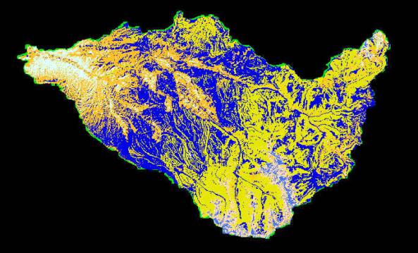 |
Image 5
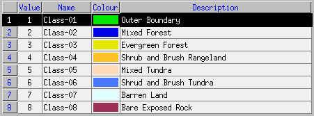 |
Table 2
In the next iteration a classification with the DEM derived channel for 'aspect' was added. The results of this classification are listed below and seen in Image 6/Table3:
1. Outer Boundary (an effect from the bitmap mask)
2. Mixed Forest
3. Evergreen Forest
4. Shrub and Brush Rangeland
5. Mixed Tundra
6. Shrub and Brush Tundra
7. Barren Land
8. Bare Exposed Rock
This classification was influenced highly by the addition of aspect and showed vegetative differences across the low, mid, and high elevations of the watershed. Field verification later confirmed that the vegetation is very homogeneous in these areas and that aspect influenced the classification as to the amount of open area and vegetative density on south and west facing slopes, as opposed to north and east facing slopes.
The next approach was to add texture as a layer along with the reflective/infrared bands and run an unsupervised classification, producing a vegetative texture image of the study area. This classification resulted in the following classes listed below and seen in Image 7/Table 4:
1. Evergreen Forest
2. Mixed Forest
3. Shrub and Brush Rangeland
4. Cropland and Pasture
5. Mixed Tundra
6. Shrub and Brush Tundra
7. Barren Land
8. Bare Exposed Rock
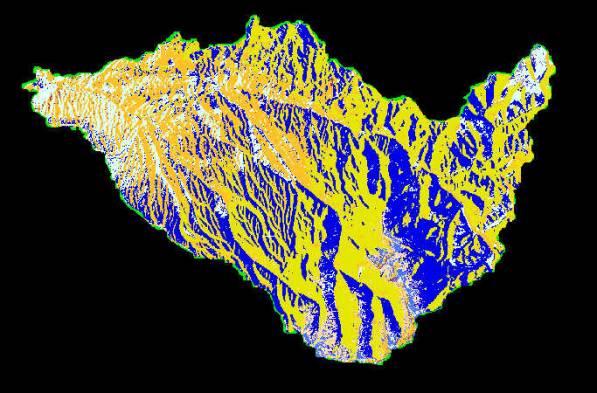 |
Image 6
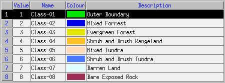 |
Table 3
These classes show a trend that relates to the straight vegetative classification in many of the land cover classes and bounds showed a similarity. The main exception is the range of evergreen forest and the barren areas showed up stronger in the lower regions and highest peaks of the watershed. This is expected because the texture filter relates the density of canopy cover for specific stands plus the height and openness of land cover.
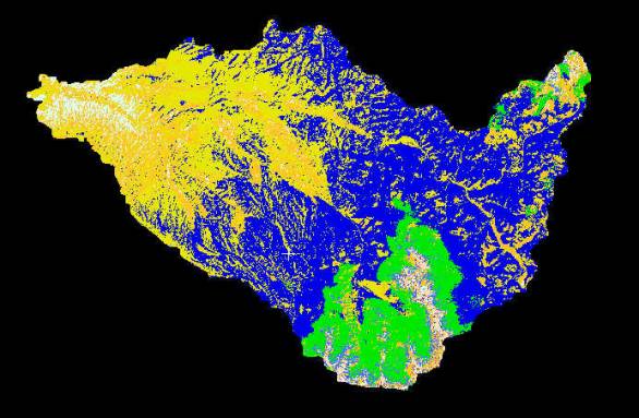 |
Image 7
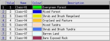 |
Table 4
The texture and reflective/infrared bands along with slope, elevation, and aspect were classed and a new image output, which showed the hydrologic attributes of these fields displayed as one eight class, classification channel. The results of this classification are found in Image 8 and listed in Table 5:
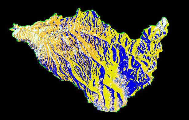 |
Image8
 |
Table 5
These classes are directly comparable to the classification of straight land cover vegetative results with the added channels of elevation, slope, and aspect. Even though texture was added the influence of aspect and elevation somewhat overpowered the addition of this band within this classification. The only exception is that there are minor changes in the highest elevations of the watershed attributed to texture.
The major vegetative classes for the five above remained steady across the study area with only minor to moderate differences attributed to hydrologic inputs. This is very promising, in that the data showed the vegetative categories assigned during the unsupervised classification, while adding the hydrology significant bands of slope, elevation, aspect, and texture. With vegetation being a major factor in any hydrology classification, the verification of the vegetation classifications are pivotal to the hydrologically significant bands. The data from the GPS verification showed that the unsupervised vegetation analysis was correct and validated the possibility of an accurate hydrology classification. This related the possibility that the classification would be an invaluable tool for later hydrologic modeling of the watershed using the new hydrology classification as opposed to a standard land cover classification.
Interpretation
During the process of this study there are many differences that contribute to the total hydrologic classification regime. The study first looked at the unsupervised classification of the Embudo watershed to derive an accurate land cover classification. These classes were grouped into eight categories and verified by GPS, maps, and expert opinion. The labels given in the classification are somewhat homogenous because the study area is very rural and contributes to land cover in a very homogenous way, with broad areas of similar or same cover types. The next step in this study was to derive a classification from the vegetative classification that would be hydrologically viable in determining classes that would be hydrologically accurate in future determinations of surface runoff. The hydrology classification was done by incorporating a standard unsupervised vegetative cover classification with added channels of elevation, slope, aspect, and texture to ascent hydrologic characteristics of the landscape. The comparison of the standard classification to that of the hydrology classification showed that elevation, slope, aspect, and texture were viable choices for a more accurate input to future hydrologic models.
The differences in the hydrological classification were compared to the straight vegetation land cover classification and differences addressed as to what features in the classification changed because the addition of hydrologically significant bands, and where in the watershed these changes occurred. The results of this comparison can be seen in (Table 6) where the multiple unsupervised classifications occupy the y-axis and the location within the watershed occupies the x-axis. The location in the watershed is broken into three groups: low-elevation vegetation change, mid-elevation vegetation change, and high-elevation vegetation change. Change is specific to the classification using bands 1,2,3,4,5 and 7 for the original land cover classification. The vegetation groups are broken into these three elevation categories because of the prevalent homogeneous vegetation types located within the classification bounds of the watershed. The added channels of DEM derived and texture derived data showed that a hydrologic classification could be more advantageous to models that would normally incorporate a standard land cover classification. The vegetative cover and on site investigation of percentage of cover and runoff potential from derived classes hold promise that the classification once incorporated into a model will produce a better estimate of runoff for the hydrologic land classes.
This hypothesis needs to be tested in hydrologic models to produce an accurate assessment of the hydrology classifications performed in this study. The final test will come when the different classifications are tested in a model and the best potential runoff evaluated for each classification and each class. It is my opinion and of others that the hydrology classes will prove to be reliable in producing better estimated runoff.
| Low Elevation Changes to Vegetation and Hydrology Compared to Land Cover Bands 1,2,3,4,5,7 |
Mid Elevation Changes to Vegetation and Hydrology Compared to Land Cover Bands 1,2,3,4,5,7 |
High Elevation Changes to Vegetation and Hydrology Compared to Land Cover Bands 1,2,3,4,5,7 |
|
| Land Cover With Landsat 7 ETM+ Bands 1,2,3,4,5,7 |
Base for Evaluation |
Base for Evaluation |
Base for Evaluation |
| Land Cover With ETM+ Bands 1,2,3,4,5,7 Plus Slope and Elevation |
More Barren Areas Present With a High Potential Runoff |
No Apparent Change Compared to Land Cover |
More Barren Areas Present With a High Potential Runoff |
| Land Cover With ETM+ Bands 1,2,3,4,5,7 Plus Slope, Elevation, and Aspect |
More Barren and Exposed Rock Areas on South and West Facing Slopes With a High Potential Runoff |
Vegetative Areas Highly Impacted by Aspect, Showing Moderate to Low Potential Runoff on South and West Facing Slopes |
More Barren and Exposed Rock Areas on South and West Facing Slopes and Peaks With a Moderate Potential Runoff |
| Land Cover With ETM+ Bands 1,2,3,4,5,7 Plus Band 2 Derived Texture |
More Barren Areas of Low Texture/ Low Canopy Cover With a High Potential Runoff |
Very Little Change Compared to Land Cover, More Apparent Mixed Forest With Low Potential Runoff |
Very Little Change Compared to Land Cover, With the Exception to Highest Barren Peaks, Low to Moderate Potential Runoff |
| Land Cover With ETM+ Bands 1,2,3,4,5,7 Plus Slope, Elevation, Aspect, and Texture |
More Barren and Exposed Rock Areas on South and West Facing Slopes With a High Potential Runoff |
Vegetative Areas Highly Impacted by Aspect, Showing Moderate to Low Potential Runoff on South and West Facing Slopes |
More Barren and Exposed Rock Areas on South and West Facing Slopes and Peaks Showing Moderate to High Potential Runoff |
Table 6
Conclusions
This study has added hydrologic parameters to classifications that were only marginal in displaying land cover for hydrologic modeling. The scientific background has related that the success of such a classification would be advantageous to modelers of overland flow. Traditional classifications as inputs to these models have acceptably been classifications of single land cover classes with no hydrologic dependent channels. These channels are elevation, slope, aspect, and texture, all of which are hydrologically important when deriving a land classification for hydrologic purposes.
The methodology of this study incorporated many aspects of remote sensing/image processing and GIS. First, the data was put into a GIS with the watershed bounds and flow-accumulation derived. The data were processed and rescaled to fit a geocorrected image of the Embudo watershed, then in Northern New Mexico. Once this was done a vegetative land cover of the area was classified in an unsupervised fashion. The unsupervised classification was then labeled according to Anderson level II classes and the vegetation across the watershed assessed. After the vegetative classes were determined, the DEM derived data was added as channels and a hydrologic based land cover classification derived. The purpose of introducing the DEM derived channels is to get a better estimation of surface runoff once incorporated into a model. The validity of the classes for vegetation and relevance of the hydrologic classification were assessed using GPS and expert ground truth verification.
The interpretation of the results looks promising and the final judgement will come once incorporated into a hydrology runoff model. The hydrologic based classification derived in this study should give a better estimate of surface runoff compared to that of a standard spectrally based vegetation classification. This is because the use of hydrologically important channels such as elevation, slope, aspect, and texture are incorporated and should yield a better runoff estimate and a more accurate model output for overland flow.
The future of hydrologic modeling and hydrology classifications should improve over time as technology improves. The addition of climate data and relevant ground sensed data should and would improve the concept of a hydrologic based land classification. If time permits the soils, evapotranspiration, river gauge data, and rain gauge data should be incorporated into future research. The emphasis in future products should be on the interpretation of the derived map, rather than on the product of the map (Mausel et al, 1990). It has been said and still holds true that future improvements in the use of satellite data to estimate forest hydrological variables will come from the following developments (Stewart and Finch, 1993).
1. Use of multitemporal satellite data.
2. Combined analysis of remotely sensed and ground based data.
3. Combined analysis of different types of remotely sensed data.
4. Improved analysis techniques.
5. Combining satellite data with models.
The additions of new sensors holds great promise for the integration of hydrology and land cover processes. With new techniques developing the science of hydrology classifications, these classifications will hopefully one day be incorporated into standard hydrologic modeling approaches.
References
Alonso, Gonzalez F. , Soria , Lopez S., (1991), Using Contextual Information to Improve Land Use Classifications of Satellite Images in Central Spain. International Journal of Remote Sensing, 1991, Vol. 12, No 11, p2227-2235
Anderson, James R., Hardy, Earnest E., Roach John T., and Witmer Richard E., (1976), (1976), A Land Use and Land Cover Classification System for Use With Remote Sensor Data. Geological Survey Professional Paper 964, US Government Printing Office, 1976
ANHIC, Land Classification System, Introduction, Alberta Environment. (2001).
(http://www.alberta/canenv/intro/gov/html)
Arc/Info grid book (surface hydrologic analysis) Environmental Systems Research Institute, (Esri), 1994
Engman, E.T., and Gurney, R.J., (1991), Remote Sensing in Hydrology. (London: Chapman and Hall)
Gregorio, Antonio D.I. and Jansen, Louisa J.M., (1996) FAO Land Cover Classification: A Dichotomous, Modular-Hierarchical Approach. (http://www.fao.org/waicent/faoinfo/sustdev/eidirect/eire0019.htm)
Kartikeyan, B., Gopalakrishna, B., Kalubarme M.H., Majumder, K.L., (1994), Contextual Techniques for Classification of High and Low Resolution Remote Sensing Data. International Journal of Remote Sensing, 1994, Vol. 15,No. 5, p1037-1051
Schultz, Gert A., Engman, Edwin T., (2001), Remote Sensing in Hydrology and Water Management. (Germany: Springer and Varlag)
Kite, G.W., (1978), Development of a Hydrologic Model For a Canadian Watershed. Canadian Journal of Civil Engineering, Vol. 5, No. 1, p126-134
Kite, G.W. and Kouwen, N., (1992), Water Modeling Using Land Classifications. Water Resources Research, Vol. 28, No. 12, p3193-3200, December 1992
Kouwen, N., Soulis, E.D., Pietroniro, A., Donald, J., and Harrington, R.A., (1993), Grouped Response Units for Distributed Hydrologic Modeling. Journal of Water Resources Planning and Management, Vol. 119, No. 3, May/June, 1993
Leavesley, G.H., and Stannard, L.G., (1990), Application of Remotely Sensed Data in a Distributed-Parameter Watershed Model. Applications of Remote Sensing in Hydrology. Feb., p47-68, 1990
Mausel, P.W., Kramber, W.J., Lee, J.K., (1990), Optimum Band Selection for Supervised Classification of Multispectral Data. Photogrammetric Engineering and Remote Sensing, Vol. 56, No. 1, p55-60, 1990
(Nasa) Landsat 7 ETM+ Platform Data, 2001 (http://landsat.gsfc.nasa.gov/project/satellite.html)
New Mexico Resource Geographic Information System, Produced by Earth Data Analysis Center, (1998)
Overview of K-means Clustering, (2001) K-means Algorithm for Unsupervised Classification. (http://www.ece.neu.edu/groups/rpl/kmeans/)
Revised IGBP-DIS LCWG Global Land Cover Classification System (February 8, 1995), International Geosphere-Biosphere Programme-Data and Information Systems Land Cover Working Group(IGBP-DIS LCWG)
(http://www.vcrlter.virginia.edu/modlers/modlc/classes.html)
Runoff and Hydrologic Modeling, (2001), US National Report to IUGG, 1991-1994, Rev. American Geophysical Union, Vol. 33. Supplement. 1995.
(http://www.agu.org/revgeophys/engman00/node8.html)
Stewart, J.B. and Finch J.W., (1993), Application of Remote Sensing to Forest Hydrology. Journal of Hydrology, 150(1993) p701-716
Swain, P.H., Siegel, H., and Smith, B.W., (1979). A Method for Classifying Multispectral Remote Sensing Data Using Context. Processing of Remote Sensing Data Report. p19-29, 1979
Thompson, Mark (1996), A Standard Land-Cover Classification Scheme for Remote Sensing Applications in South Africa. South African Journal of Science, Jan96, Vol. 92 Issue 1, p34, 9p, 4charts
Townsend, John R.G., (1984), Agriculture Land-Cover Discrimination Using Thematic Mapper Spectral Bands. International Journal of Remote Sensing, 1984, Vol. 5, No. 4, 681-698
United States Geological Survey (USGS), (2001), Land Cover Classification Codes. (http//www.usgs.gov)
Wilson, Mike, (1997) Using DEM's in an Unsupervised Classification. (http://gis.mursuky.edu/gsc/gsc641/1997/wilson/)