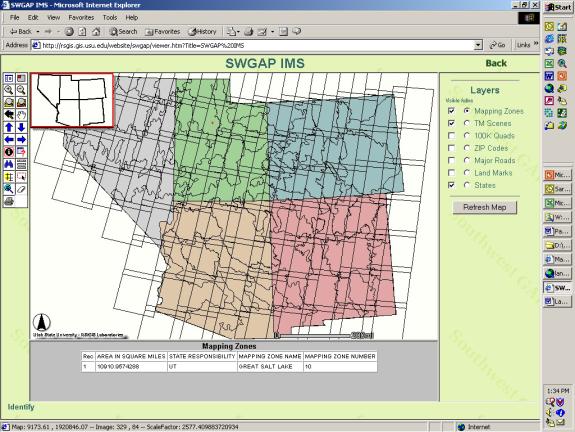
Figure 1. Southwest region showing mapping zone and state responsibilities
The Southwest Regional Gap Analysis Project (SWReGAP) is a coordinated effort to complete a Gap Analysis (USGS-BRD) for a large area encompassing the states of Arizona, Colorado, New Mexico, Nevada and Utah. One of the key products from this effort will be a seamless coverage of vegetative land cover modeled from Landsat 7 imagery and ancillary GIS data. This paper presents an overview of the 5-state effort, and focuses on the role of GIS throughout various aspects of the project. Specifically GIS has been used extensively for field data collection, data management, data automation, data generation and modeling.
The mission of the Gap Analysis Program (GAP) is to develop and provide large landscape-scale geographic information on biological diversity to planners, land managers and policy makers for informed decision-making (USGS GAP, 2002). GAP is managed and directed by the Biological Resources Division of the U. S. Geological Survey (USGS-BRD). One of the traditional goals of gap analysis lies in identifying spatial "gaps" in biodiversity protection. Gaps are determined by overlaying land stewardship maps over potential vertebrate habitat distribution maps, or wildlife habitat relationship models (WRMS). A key input to the WRMS is vegetative land cover.
During the 1990s several western states completed gap analyses on a state-based model. That is, each state developed and compiled vegetative land cover, WRMS and land stewardship GIS data layers for their own state. Along with the traditional gap analysis, vegetation land cover and WRMS GIS datasets were distributed as stand-alone products on CD-ROM to be used by planners and land managers.
The Southwest Regional Gap Analysis Project (SWReGAP) is the first formalized cooperative gap analysis project to be conducted at a regional level, and includes the states of Arizona, Colorado, New Mexico, Nevada and Utah. The 5-state region encompasses approximately 560,000 square miles. SWReGAP follows the state-based business model by dividing some responsibilities and funding among individual state teams. However, in order to assure standardization across the region, four fundamental measures have been undertaken. First, regional laboratories have been established to provide direction and develop protocols that are to be followed by cooperating states.
For vegetative land-cover mapping, the regional lab is at Utah State University, while the animal modeling regional lab is at New Mexico State University. Second, all states are using the same source data for image classification and land cover mapping. These data include Landsat TM 7 imagery for three seasons (spring, summer and fall) for the entire region. Two hundred and forty TM scenes from 1999, 2000 and 2001 were purchased through the Multi-Resolution Landscape Characteristics program at USGS Eros Data Center. Ancillary data for the 5-state region includes 30 meter DEMs and derivatives (slope, aspect, landform). Third, a single target land cover legend for the 5-state region has been established and is being coordinated by NatureServe (formerly with the The Nature Conservancy). The legend is based on the National Vegetation Classification System (NVCS), recommended as the standard by the FGDC for federally funded vegetation mapping projects (FGDC 1997). Fourth, rather than divide the region by political boundaries (i.e. state lines) mapping responsibilities are distributed among the five states along ecological and physiographic boundaries. In order to facilitate the remote sensing based mapping, the 5-state region has been divided into 73 ecologically meaningful mapping zones (Figure 1), which have been subsequently divided into five regions of state responsibility.
Figure 1. Southwest region showing mapping zone and state responsibilities
Remote sensing-based mapping using satellite imagery is the most feasible method for mapping large geographic areas such as the 5-state region in this project. Since the 1970s remote sensing scientists and land cover mapping practitioners have been developing new and better techniques for remotely sensed-based mapping. An important contribution of the gap analysis program to the remote sensing-based mapping discipline has been the development of a variety of methodologies for land cover mapping (Eve and Merchant 1998). Various methodologies have been employed through many state-based GAP projects, as well as other large landscape mapping projects. Eve and Merchant (1998) conducted a survey of land cover mapping protocols used by state-based projects in the Gap Analysis Program. Recommendations from the Eve and Merchant report provided the foundation upon which many of the methodologies for the Southwest Regional GAP project were developed.
Physiographic/Ecological Stratification
Stratifying the landscape by physiographic and ecological characteristics provides an effective means to 1) improve the efficiency by which spectral modeling, and ultimately land cover mapping can be accomplished and 2) partition the landscape into manageable working units. Spectral classification of satellite imagery involves the effective identification of spectral gradients resulting from the variability of physiographic and phenologic variables, ground variability, as well as solar and atmospheric influences within and between remotely sensed imagery. Stratifying the landscape based on similar physiographic and ecological characteristics provides a means by which spectral differentiation is maximized within areas of uniform ecological characteristics. Lillisand (1996) refers to these units as "spectro-physiographic areas" or "spectrally consistent classification units (SCCUs)." Within the SWReGAP project these ecoregional units are referred to as mapping zones (Figure 1).
Overview of Rule-Based Mapping
Rule-based image classification capitalizes on the availability of multiple spatial modeling datasets, and the recognition that other "ancillary" datasets, independent of the remotely sensed imagery provide valuable information that can be used to more effectively map vegetative land cover. The premise of a rule-based modeling approach is that distinct vegetation communities are associated with different ranges of environmental and spectral gradients, and that "rules" can be drawn from spectral and ancillary modeling layers to correctly identify the spatial distribution of target vegetation communities.
A rule is a series of conditional statements that identify the range of values in each modeling dataset that define the target vegetation community. A simple example of a classification rule is as follows:
CONDITION {elevation > 2000 AND SprNDVI > 0.55 and SprNDVI < 0.90 AND landform = 6} THEN Douglas Fir
Rule-based mapping is conducted at the pixel level. With the above example, pixels in the resulting classification image are assigned a value representing Douglas Fir when pixels in the input datasets (elevation, SprNDVI and landform) meet the criteria in the rule.
Spatial Data Modeling Layers
The availability of relatively inexpensive satellite imagery, and extensive coverage of digital elevation model (DEM) data for the conterminous United States, provide a significant number of spatially explicit modeling data to be used for the vegetation mapping process. Landsat TM 7 imagery for three seasons (spring, summer and fall) were purchased through the Multi-Resolution Landscape Characteristics (MRLC) Consortium and 30 meter DEM data obtained from the National Elevation Database. From these two sources several core modeling datasets are being created for rule-generation (Table 1). Data layers are generated for each mapping zone. Landsat TM imagery is mosaicked and clipped to the mapping zone boundary, and derivative layers such as NDVI (Normalized Difference Vegetation Index) and Tassel-Cap bands (brightness, greenness and wetness images) are created. DEM derivatives are generated using ArcInfo Grid, or AML programs, such as in the case of the Topographic Relative Moisture Index and Landform. A 2000 meter buffer beyond the mapping zone is included to facilitate edge-matching between mapping zones when the final vegetation classification is complete.
| Derived from Landsat TM imagery | Derived from Digital Elevation Model |
| Spring NDVI | Slope |
| Spring Brightness | Aspect |
| Spring Greenness | Elevation |
| Spring Wetness | Topographic Relative Moisture Index |
| Summer NDVI | Landform |
| Summer Brightness | |
| Summer Greenness | |
| Summer Wetness | |
| Fall NDVI | |
| Fall Brightness | |
| Fall Greenness | |
| Fall Wetness |
Field Data Collection
Percent canopy cover and species dominance of target vegetation communities in the landscape are collected in the field using ocular estimation. In addition, the geographic location of sample sites is collected using a GPS and digitized over geo-referenced imagery using a laptop computer. Vegetation communities are subsequently given an appropriate label in accordance with the National Vegetation Classification System (Grossman et al. 1998).
Rule Generation
Decision trees have been used to generate modeling rules in several remote sensing-based mapping projects (Larwrence & Wright 2001, Hansen et al. 2000, Friedl & Brodley 1997, Hansen, Bubayah & Defries 1996). Decision trees, also known as CART (Classification and Regression Trees) are exploratory tools that can be used to identify complex interactions amongst numerous variables (Venables and Ripley, 1999). A decision tree requires a single dependent variable (e.g. vegetation cover type) and multiple independent variables (e.g. DEM derived and imagery derived datasets). The result of a decision tree analysis is the generation of rules that correspond to "branches" of the decision tree (Figure 2). S-PLUS is used for generating the CART, and output from S-PLUS is reformatted to a modeling language (.mdl file) suitable for model generation using ERDAS Imagine software.
Figure 2. Example of decision tree graphic created in S-PLUS
Map Validation and Edge-matching
The process of generating land cover maps for each mapping zone is an iterative process involving modifying and adjusting rules to produce the most correct land cover map possible. Validation of model rules and the resulting land cover map is assessed by a 10-fold cross validation during the CART modeling process, and by intersecting withheld, or additional, field sample sites through the classified image. The results of this intersect are analyzed within a cross-tabulation matrix to determine the validity of the classification. When a land cover dataset is complete for a given mapping zone it is joined to completed land cover datasets for adjacent mapping zones. Because each mapping zone is created using a 2000 meter buffer, an area of approximately 4000 meters is available for "adjustment" of cover type boundaries in order to edge-match the mapping zones properly.
While the SWReGAP effort is essentially a remote sensing-based mapping project, GIS, and Esri products in particular, have been used extensively throughout. GIS has been used to develop specific geo-spatial tools for field data collection, data analysis and data modeling. The role of GIS has also included the development of tools for data management, regional coordination and other miscellaneous tasks. Table 2 provides an overview of GIS tools and tasks performed with the aid of GIS that are presented in greater detail later in this paper.
| Tool/Method Name | Type of Task | Esri software |
| Fld3v6.avx | Field data collection | Arcview (extension) |
| Extract_mzelev.aml | Data management | ArcInfo (aml) |
| Mz_clipcov.aml | Data management | ArcInfo (aml) |
| Zonalintersect.aml | Data analysis | ArcInfo (aml) |
| Site_intersect.aml | Data analysis | ArcInfo (aml) |
| Samples.aml | Data analysis | ArcInfo (aml) |
| Trmim.aml | Data modeling | ArcInfo (aml) |
| Landform.aml | Data modeling | ArcInfo (aml) |
| SWReGAP Data IMS | Regional Coordination | ArcIMS |
Field Data Collection
The field data collection tool has two primary functions. First, it aids in assuring the correct geographic location of the field sample site and allows the user to record the location of the site digitally while in the field. Second, and perhaps more importantly, it allows the field crew to view the field site location from a birds-eye perspective using the same imagery that will be used for image classification.
Field crews take with them a laptop computer with ArcViewTM and the field data collection extension (fld3v6.avx) installed, as well as TM imagery (Figure 3) or a landform stratification image (Figure 4) for the mapping zone. Other GIS datasets such as roads, landownership, geology, etc. may also be used for orientation purposes. The extension works by prompting a user for a UTM coordinate pair, and then zooming in to that location at a specified scale. The user is then prompted to digitize a polygon and enter a site ID number. The data are saved as a shapefile. The tool also contains several checks such as assuring that the user does not enter a site ID twice, and automatically converts all character entries to capitals. Insuring a systematic entry system for the site ID is critical, as the shapefiles are eventually linked to tabular data in an Access database using the site ID field.
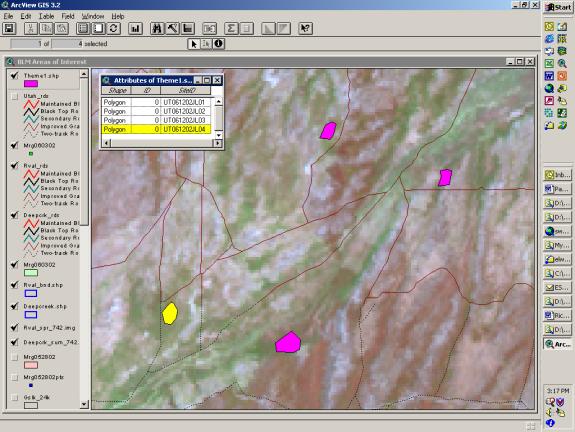
Figure 3. ArcView field data collection tool with TM imagery as backdrop
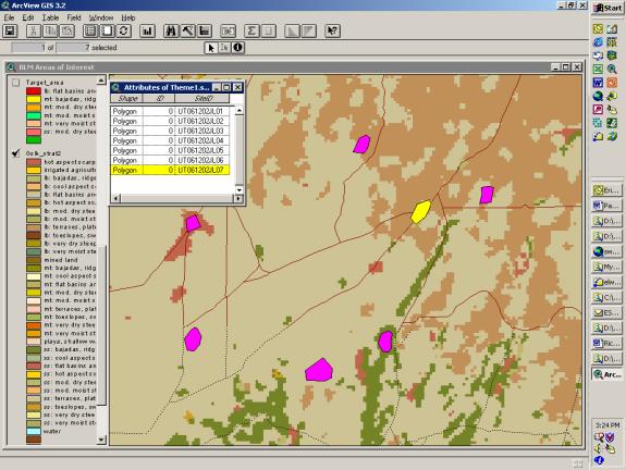
Figure 4. ArcView field data collection tool with landform stratification
image as backdrop
Data Management
An efficient way to eliminate potential errors when working with GIS software and data is to automate frequently performed tasks. Using the mapping zone as the functional working unit, ArcInfo AML tools were developed to facilitate frequently performed operations on mapping zones. Two of these are the EXTRACT_MZELEV and the MZ_CLIPCOV AMLs. These AMLs and all AMLs for the project were set up as an Atool directory, which allowed multiple users to access the AMLs as ArcInfo commands. EXTRACT_MZELEV allows a user to specify one of the 73 mapping zones and clip out an elevation grid from a master grid for the entire region. A similar command is the MZ_CLIPCOV AML, which creates a clip coverage for a specified mapping zone.
Related to data management tools are data management methods, or protocols. Over 200 GB of vector and raster (mostly raster) data are in use at any one time, and an orderly directory structure is essential. Polygon data retrieved from the laptop computers must be downloaded weekly and archived in an orderly fashion until needed. Figure 5 provides a schematic of the directory structure being used.
Figure 5. Data directory organization for Utah SWReGAP geo-spatial data
Data Analysis
ZONALINTERSECT and SITE_INTERSECT tools
The ZONALINTERSECT tool is used to intersect the field site polygons through a list of predictor variable data layers (Figure 6). The mean value for continuous predictor variables and the majority value for categorical variables are determined for each field site polygon and recorded as a separate record in the resulting output .dbf file (Figure 7). ZONALINTERSECT uses ArcInfo Grid's ZONALSTATS function to determine the mean or majority values, which allows a user to make use of all the statistics options (MAX, MIN, SUM, STD, etc.) within the ZONALSTATS function, in addition to the mean and majority statistics.
Figure 6. Scematic of ZONALINTERSECT
Figure 7. Output .dbf file of ZONALINTERSECT
The SITE_INTERSECT tool performs essentially the same function as the ZONALINTERSECT command, with the exception that it intersects the field site polygons through a single grid as opposed to a list of grids.
SAMPLES tool
The SAMPLES tool is used to determine the number of target field samples by strata for a given mapping zone using a stratified sampling approach. Typically the stratification dataset used is a landform grid, but any categorical raster dataset can be used. Input for the SAMPLES command is the stratification grid and a target number of total samples for the grid. As a result of running the command, a table is produced identifying the percent and total acres within the grid for each category. In addition, the table identifies the number of samples that would have to be collected in proportion of the area for each stratification category within the mapping zone.
| GSLK Stratification by landform/lifezone | |||
| Proportion of mapping zone | |||
| STRATA | PERCENT | ACRES | APPROX. # OF SAMPLES OF 500 TOTAL |
| 0 | 0.00 | 15314531.50 | 0.0 |
| 1 | 4.05 | 255688.70 | 20.2 |
| 2 | 0.48 | 30594.64 | 2.4 |
| 3 | 7.24 | 457073.03 | 36.2 |
| 4 | 19.73 | 1245661.19 | 98.7 |
| 5 | 0.16 | 10394.29 | 0.8 |
| 6 | 0.87 | 55020.49 | 4.4 |
| 7 | 0.85 | 53467.95 | 4.2 |
| 8 | 0.09 | 5969.30 | 0.5 |
| 9 | 0.00 | 190.81 | 0.0 |
| 10 | 0.01 | 375.85 | 0.0 |
| 11 | 1.39 | 87484.58 | 6.9 |
| 12 | 0.40 | 25500.68 | 2.0 |
| 13 | 12.80 | 808056.60 | 64.0 |
| 14 | 9.74 | 614982.95 | 48.7 |
| 15 | 1.20 | 75600.69 | 6.0 |
| 16 | 4.26 | 269261.24 | 21.3 |
| 17 | 5.33 | 336430.94 | 26.6 |
| 18 | 0.66 | 41373.01 | 3.3 |
| 19 | 0.08 | 4961.85 | 0.4 |
| 20 | 0.13 | 8154.33 | 0.6 |
| 21 | 0.08 | 4803.51 | 0.4 |
| 22 | 0.14 | 8774.81 | 0.7 |
| 23 | 3.00 | 189087.00 | 15.0 |
| 24 | 0.28 | 17800.04 | 1.4 |
| 25 | 1.30 | 81974.08 | 6.5 |
| 26 | 3.13 | 197901.18 | 15.7 |
| 27 | 2.81 | 177356.79 | 14.0 |
| 28 | 0.29 | 18594.88 | 1.5 |
| 29 | 0.31 | 19338.35 | 1.5 |
| 30 | 0.25 | 15918.13 | 1.3 |
| 31 | 13.04 | 823069.59 | 65.2 |
| 32 | 5.64 | 356260.78 | 28.2 |
| 34 | 0.26 | 16269.52 | 1.3 |
Data Modeling
Two modeling programs were created using AML and ArcInfo Grid. Using an elevation grid as input the TRMIM tool creates a Topographic Relative Moisture Index (TRMI) grid. The TRMI is a summed scalar index of four landscape elements derived from the DEM. These elements are relative slope position, slope angle, slope shape and slope aspect. The TRMIM tool developed for this project was a modified version of work done by Parker (1982) who conceived the idea of a TRMI, and Haplin (1999) who created an ArcView tutorial for the TRMI.
The TRMI grid generated by the TRMIM.AML is a grid of potential relative moisture. Index values range from 1 to 28 (drier to wetter) and are relative in the sense that pixels have the potential to be either wetter or drier relative to surrounding pixels based on slope angle, slope shape, aspect, landscape position (Figure 8).
Figure 8. Topographic Relative Moisture Index (0-27; dryer to wetter)
LANDFORM.AML is the second modeling tool used by the project, and requires a slope grid and a TRMI (0-27 classes) grid as input. The LANDFORM model reclassifies a TRMI grid based on index value and slope limits (Table 4). As a result of running the LANDFORM model, a grid with 10 Landform Position Classes (LPC) is created (Figure 9).
| Landform Position Class | Slope Limit | Refined TRMI | |
| 1 | Valley flats | lt 3 degrees | TRMI lt 22 |
| 2 | Gently sloping toe slopes, bottoms, and swales | 3-10 degrees | TRMI gt 18 |
| 3 | Gently sloping ridges, fans, and hills | 3-10 degrees | TRMI le 18 |
| 4 | Nearly level terraces and plateaus | lt 3 degrees | TRMI le 22 |
| 5 | Very moist steep slopes | 3-10 degrees | TRMI ge 18 |
| 6 | Moderately moist steep slopes | 10-35 degrees | TRMI 11-18 |
| 7 | Moderately dry steep slopes | 10-35 degrees | TRMI 4-11 |
| 8 | Very dry steep slopes | 10-35 degrees | TRMI lt 4 |
| 9 | Cool aspect scarps, cliffs, canyons | gt 35 degrees | TRMI gt 10 |
| 10 | Hot aspect scarps, cliffs, canyons | gt 35 degrees | TRMI lt 11 |
Figure 9. Ten class Landform Position Classes using LANDFORM
Regional Coordination
Due to the regional nature of the SWReGAP project, the development of an Internet Map Server that could be used to display basic vector datasets was helpful. Occasionally as state coordinators need to discuss spatial features such as where a mapping zone lies in relation to a Landsat TM scene, the ability to go to the internet to and query project data proved helpful.
Availability of GIS Tools
The ArcView extension and the AMLs presented in the paper are available for download at http://www.gis.usu.edu/~jlowry/swregap/. Note that these tools are provided without warranty of any kind, either expressed or implied, and the RSGIS Lab, nor Utah State University is responsible for the proper or improper use of these tools.
Anticipated Products from SWReGAP
The anticipated completion data for the SWReGAP project is June, 2004. While a complete description of how the data will be available to the public is not yet available, it is anticipated GIS data will be published on CD-ROM and will be available through the internet. Geo-Spatial data that will be available for the 5-state region include at a 30 meter resolution:
An interactive data-delivery system is in consideration as a vehicle by which the resulting data can be easily queried and manipulated by the user. The data-delivery system will be designed using Esri MapObjects ä and will be designed to work with ArcView 8.X.
While the land cover mapping portion of SWReGAP is primarily a remote sensing-based mapping effort, it is evident from this paper that GIS software plays a very important role as well. Remote sensing-based mapping projects rely heavily on the image processing capabilities of software such as ERDAS Imagine. In this project, for example, ERDAS Imagine is being used for scene standardization prior to mosaicking, and the mosaicking and subsetting of imagery to mapping zones. Image processing software is also indispensable in the creation of imagery derived transformations such as the NDVI and Tassel-cap bands. Furthermore, Imagine's raster modeling capabilities have proved important in the final image classification using classification rules.
Nevertheless, GIS software makes a crucial contribution to the overall project for several reasons. First, GIS software is capable of handling both vector and raster spatial datasets sufficiently well to make data management tools for both raster and vector datasets possible. Second, GIS software is easier to customize. Programming languages such as Avenue and AML are relatively easier programming tools to learn and use than those available with Imagine (i.e. C-Toolkit). And third, GIS software, particularly ArcViewä, are relatively less expensive than software dedicated to specialized tasks such as image processing.
Eve, M. and J. Merchant. 1998. A national survey of land cover mapping protocols used in the gap analysis program. Final Report. Internet WWW page, at URL: http://www.calmit.unl.edu/gapmap/report.html
FGDC (Federal Geographic Data Committee), 1997. Vegetation classification standard, FGDC-STD-005. Internet WWW page, at URL: http://www.fgdc.gov/Standards/Documents/Standards/Vegetation.
Friedl, M. A. and C. E. Brodley. 1997. Decision tree classification of land cover from remotely sensed data. Remote Sensing of the Environment. Vol. 61: 399-409.
Grossman, et al. 1998. D. H., D. Faber-Langendoen, A. S. Weakley, M. Anderson, P. Bourgeron, R. Crawford, K. Goodin, S. Landaal, K. Metzler, K. Patterson, M. Pyne, M. Reid, and L. Sneddon. 1998. International Classification of Vegetation Communities: Terrestrial Vegetation of the United States: Volume 1, The National Vegetation Classification System: Development, Status, and Applications. Arlington, VA: The Nature Conservancy.
Hansen, M. C., R. S. DeFries, J. R. Townsend and R. Sohlberg. 2000. Global land cover classification at 1 km spatial resolution using a classification tree approach. International Journal of Remote Sensing. Vol. 21, No. 6 & 7, pp 1331-1364.
Hansen, M. , R. Dubayah and R. DeFries. 1996. Classification trees: an alternative to traditional land cover classifiers. International Journal of Remote Sensing. Vol 17, No. 5, pp 1075-1081.
Haplin, P. N. 1999 "GIS analysis for conservation site design: A short-course developed for The Nature Conservancy." Nicholas School of the Environment-Landscape Ecology Lab, Duke University.
Lawrence, R. and A. Wright. 2001. Rule-based classification systems using Classification and Regression Trees (CART) Analysis. Photogrammetric Engineering and Remote Sensing. Vol. 67, No. 10.
Lillisand. T. M. 1996. A protocol for satellite-based land cover classification in the upper Midwest. Gap Analysis: A Landscape Approach to Biodiversity Planning. Editors J. Michael Scott, Timothy H. Tear and Frank W. Davis. ASPRS, 320 pp.
Parker, A. J. 1982. The topographic relative moisture index: An approach to soil-moisture assessment in mountain terrain. Physical Geography. 3: 160-168.
USGS GAP (Gap Analysis Program), 2002. Mission statement. Internet WWW page, at URL: http://www.gap.uidaho.edu/About/MissionStatement.htm. June 2002.
Venables, W. N. and B. D. Ripley, 1999. Modern Applied Statistics with S-PLUS, 3rd Edition, Springer-Verlag, New York, NY.
John Lowry, R. Douglas Ramsey, Gerald Manis
jlowry@cnr.usu.edu
Remote Sensing/GIS Laboratory, College of Natural Resources,
Utah State University, UMC 5275 Old Main Hill, Logan, Utah 84322-5275