Coextensive LIDAR and preliminary INSAR digital elevation models (DEMs), with extensive ground control, allow comparison of the two technologies in a well-watered suburban terrain of the Snoqualmie valley east of Seattle Washington. Terrain and land cover datasets are used to categorize the areas in which the DEMs differed. A dense network of control points is also used to categorize the error in each DEM. The patterns of disparity and error are largely as expected given the strengths and weaknesses of the two technologies.
Collection of high-resolution digital elevation models (DEMs) using airborne active sensors is increasing rapidly as these sensor systems become more widely available and cost-effective (King 2002, Maune 2001). These technologies include LIDAR (LIght Detection And Ranging, also known as airborne laser scanning) and INSAR (INterferometric Synthetic Aperture Radar, also known as IfSAR). Each technology has strengths and weaknesses and is better suited for different applications (Maune 2001, Fowler 2001, Hensley et al. 2001).
A handful of studies have made comparisons of DEMs made by these two technologies over the same region. Several groups have studied an area in Baden-Wurttemberg, Germany, which includes a 500 hectare “DTM Test Area” set up with reference and control points (Mercer and Schnick 1999, Sties et al. 2000, Mercer 2001, Dowman and Fischer 2001). The Morrison, Colorado quadrangle west of Denver has been studied extensively (Mercer 2001, Osborn et al. 2001). Brügelmann and Lange (2001) compared DEMs made along dike systems in the Netherlands. Part of the Red River valley in North Dakota and an urban area in Denver have also been examined (Mercer and Schnick 1999).
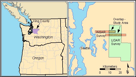
The present study compares LIDAR and INSAR surveys of areas in the Snoqualmie River valley east of Seattle, Washington (Figure 1). The test areas are suburban to rural, with modest local relief, local steep slopes, vegetation that ranges from pasture and cropland to extensive dense evergreen and mixed evergreen-deciduous forest watered by 1 to 2 m of annual rainfall. Elevations range from 6 to 200 meters. The dense vegetation of the Pacific Northwest differentiates this test site from the drier ones studied by others, as the heavy canopy tests the systems ability to acquire the ground surface. This study is also differentiated from the other comparisons by the extensive ground control in the test areas – over 1900 points.
LIDAR and INSAR are both active sensors emitting a pulse of energy and recording its return at the sensor. LIDAR uses a rapidly pulsed laser rangefinder mounted in a light aircraft with accompanying differential GPS and INS (inertial navigation system) to locate and orient the aircraft. Ten thousand to 30,000 XYZ points are surveyed per second with a spatial precision of a few decimeters, at a cost of a few hundredths of a cent per point. Flying height is on the order of 1,000m and airspeeds are on the order of 100 knots. The surveyed points include ground, vegetation, and structures, and require extensive filtering to extract usable terrain models. In heavily vegetated areas LIDAR systems can be challenged to locate the ground surface. Most LIDAR systems use a near-infrared laser that does not penetrate fog or rain. (Fowler 2001)
INSAR bypasses some of these problems. Flying higher and faster than most LIDAR systems, an INSAR-equipped plane can cover large areas. Longer (cm to m) wavelengths penetrate fog and rain. Extensive development work has resulted in systems that process data almost as rapidly as it is acquired. Unfortunately there are wave-length related tradeoffs: longer, ~0.5 m (P-band) wavelengths with the potential to penetrate vegetation to the ground of necessity lack high spatial resolution; wavelengths of a few cm (X-band) provide better spatial resolution but image the tree tops. (Hensley et al. 2001)
This analysis makes use of five datasets: an INSAR DEM (8.2 ft = 2.5m postings), a LIDAR DEM (5m postings), and ground control established with GPS, Landsat TM (28.5m postings) land cover layer and the USGS 10m DEM.
In 2001 King County contracted for two test patches of INSAR topographic survey data, as a pilot for possible production of a high-resolution digital elevation model for the county. The contractor acquired single-pass X-band and two-pass P-band interferometric SAR data in late July – early August 2001, and delivered initial ground-surface models (P- and X-band surveys combined with a proprietary algorithm) and canopy-top surfaces (X-band only survey) three weeks later.
The original INSAR ground-surface model that was delivered did not meet vertical accuracy specifications. The contractor reprocessed the P- and X-band surveys to a revised ground surface model that is examined here. This dataset is still considered preliminary and the area is currently being reflown to produce a final dataset.
The INSAR data was delivered in Washington State Plane North projection, HPGN datum. The data was collected referencing ellipsoid heights and translated to NAVD88 using GEOID99. The other datasets described below match were reprojected and resampled to match the projection, datum, and grid cell size of the INSAR dataset.
The U.S. Geological Survey (USGS) contracted a LIDAR survey in the same general area. The contractor flew the area in early September 1999 at the time of late summer low water in the Snoqualmie River. The survey was designed to put a laser pulse on the ground (or canopy) every 5 meters across and along the flight path and the area was double-flown, leading to an initial survey density of about 0.3 pulses/m2. The vegetation-filtering algorithm used to process these data to a bare-earth surface is unknown. USGS purchased filtered bare-earth points and a 5-m DEM interpolated from the bare-earth points. Data from this survey were released to the public in May 2001.
The LIDAR data was delivered in UTM Zone 10, datum NAD83. To put the data in the same projection and on the same datum as the INSAR data, we converted the LIDAR bare-earth points to a point coverage, projected the points, converted the points to a triangulated irregular network (TIN), and then gridded the TIN at 2.5 m postings to match the INSAR data.
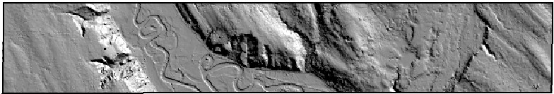
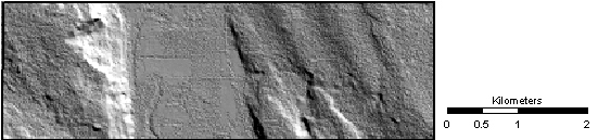
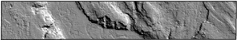
There is a 3590 hectare overlap – over 5.8 million 6.25m2 cells (2.5m on center) – between the LIDAR and INSAR surveys, in two separate patches (Figures 1 and 2).
Figure 2. a. Hillshade images of LIDAR DEMs.
b. Hillshade images of INSAR DEMs.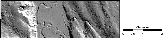
To better evaluate the INSAR data, King County established extensive ground control (~3,200 points) via survey-grade differential GPS, real-time kinematic GPS, and total-station techniques. Besides the density of this data set, it is remarkable for two features. First, all points were measured specifically for evaluating remotely-sensed DEMs; all are located on planar surfaces, not curbs, building margins, or other corners in the landscape. Second, many of the ground control points were measured by total-station offset from GPS locations, permitting precise surveying of ground elevations beneath dense canopy. In previous work we have been stymied by the tendency to use only GPS for ground control, with the result that all control points are in open areas.
There are 1906 control points in the area of overlap between the INSAR and LIDAR surveys. Table 1 shows the distribution of the control points by land cover category, and the control point locations are shown in Figure 1.
Table 1. Distribution of control points
| Land cover category | # of control points |
| Bare | 1 |
| Developed (high density) | 20 |
| Developed (low density) | 160 |
| Forest (conifer) | 81 |
| Forest (mixed) | 444 |
| Grass | 461 |
| Marsh | 144 |
| Scrub | 591 |
| Water (shallow – river) | 4 |
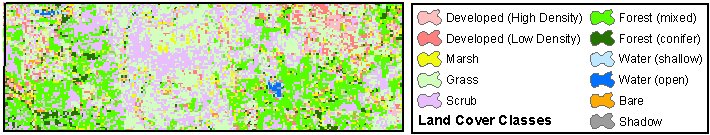
To evaluate the effect of land cover on the accuracy of different survey techniques, we used land cover data derived from a Landsat TM image. The image was acquired on August 2, 1998. The image was classified using a hybrid supervised/unsupervised approach, which yielded 12 land cover classes (PRISM 2000). Table 2 shows the land cover categories and their percentage of the study area, and Figure 3 is a map of the study area by land cover.
Table 2. Land cover in study area
| Land cover category | Percent of Study Area |
| Bare | 0.2% |
| Developed (high density) | 1.7% |
| Developed (low density) | 5.4% |
| Forest (conifer) | 7.1% |
| Forest (mixed) | 26.4% |
| Grass | 18.8% |
| Marsh | 6.1% |
| Scrub | 32.4% |
| Shadow | 0.3% |
| Water (open – lake) | 0.2% |
| Water (shallow – river) | 1.4% |
Figure 3. Land cover in study area
We used the 10-meter resolution DEM in UTM projection from the USGS as an independent source to evaluate the effects of terrain on the LIDAR and INSAR data. This DEM was produced by interpolation from standard 1:24,000-scale contour maps using LT4X software. In this area, the source maps have a 20-foot contour interval.
Slope, aspect, and curvature were all derived from the 10m DEM. These derived parameters were then projected into State Plane coordinates. The slope and aspect coverages were combined into a “terrain category” coverage with nine categories (flat – < 5% slope, and 5 to 25% slope and > 25% slope for four aspects). Table 3 shows the distribution of these terrain categories across the study area.
Table 3. Terrain characteristics in study area
| Terrain category | Percent of Study Area |
| Flat (< 5% slope) | 69.8% |
| Mid-slope North aspect | 4.4% |
| Mid-slope East aspect | 8.9% |
| Mid-slope South aspect | 6.4% |
| Mid-slope West aspect | 9.1% |
| Steep slope North aspect | 0.36% |
| Steep slope East aspect | 0.49% |
| Steep slope South aspect | 0.39% |
| Steep slope West aspect | 0.27% |
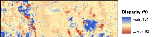
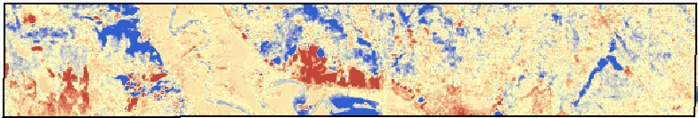
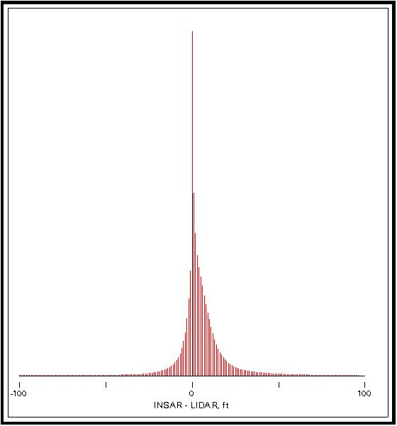
To determine the overall characteristics of the data sets, we generated an elevation disparity (INSAR elevation minus LIDAR elevation) dataset (Figure 4). We use the term ‘disparity’ to reflect that the two DEMs are being compared to each other rather than to a source of higher accuracy, such as control point elevations (where we use the term ‘error’). This disparity grid enabled some general conclusions to be drawn on the differences between the two elevation models. Figure 5 is the histogram for the INSAR-LIDAR disparity dataset. The skewness measures for the distribution are all positive (Sk = 7.35, Sm = 3.92, Sq = 24.5), reflecting the overall tendency of INSAR-derived elevations to be greater than LIDAR-derived elevations.
Figure 4. Disparity between INSAR and LIDAR DEMs
Figure 5. Histogram of disparity distribution
(INSAR minus LIDAR)
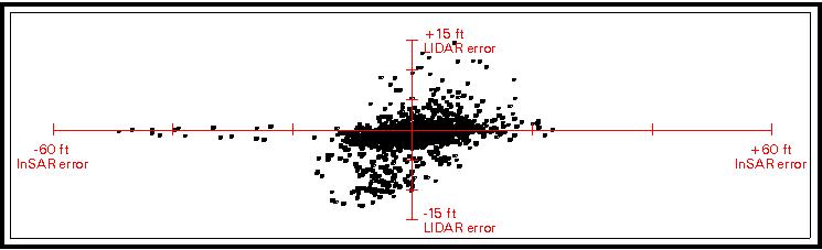
We also compared the control points and the individual INSAR and LIDAR surface models. The elevations were cross-tabulated with each surface model and the land cover dataset. Table 4 gives basic statistics for three differences: (a) the disparities between the two surface models; (b) the error in the INSAR DEM compared to the ground control points; and (c) the same for the LIDAR DEM. Note that column (a) is a comparison of two grids representing over 5.8 million cells, but (b) and (c) are comparisons between 1906 control-point elevations and the respective grid cells in each DEM. Figure 6 is a scatter plot of the control heights against the two surveys, and reflects the much higher variance of the INSAR data relative to the control points.
Table 4. Summary of disparity and error between DEMs and ground control (feet)
|
(a) INSAR – LIDAR> disparity | (b) Control – INSAR error |
(c) Control – LIDAR error | |
| Mean | 4.5 | -1.66 | -.88 |
| Standard Deviation | 14.1 | 10.80 | 2.75 |
| Maximum | 131 | 53.7 | 12.7 |
| Minimum | -192 | 63.8 | -14.7 |
The INSAR and LIDAR elevation disparity dataset was cross-tabulated with the terrain category, curvature, and land cover datasets. Bar charts showing the results are in Figures 7, 8 and 9.
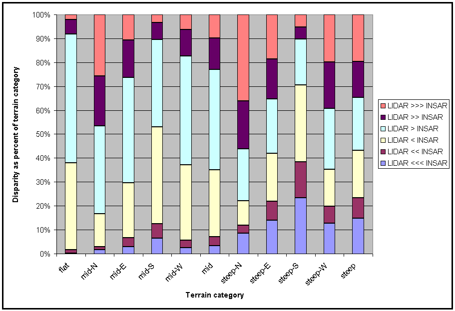
Figure 8. INSAR-LIDAR disparity versus curvature
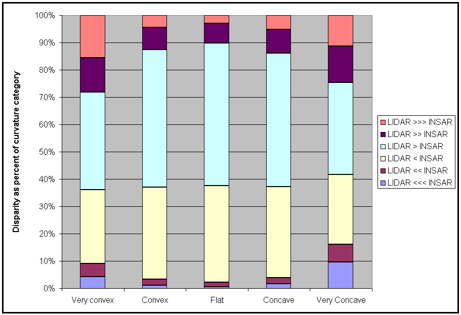
Figure 9. INSAR-LIDAR disparity versus land cover
An analysis of these bar charts yields some interesting insights into the nature of the errors in each DEM.
Looking first at the overlay of terrain categories with the DEM disparity (Figure 7), surveys disagreed more as the slope steepened. INSAR tended to report higher elevations than LIDAR on the north-facing slopes while LIDAR tended to report higher elevations than INSAR on south-facing slopes. In the flat terrain, both survey models correspond reasonably well.
Figure 8 depicts DEM disparity with curvature, another measure of terrain. Not surprisingly, the two models have greater disparity on slopes that are not flat. The INSAR DEM tends to be higher than the LIDAR DEM on concave slopes (gullies, etc.) whereas the LIDAR DEM tends to be higher on convex slopes (ridges, etc.). This suggests that, overall, INSAR acquisition and processing tends to smooth the landscape, filling in hollows and rounding off convexities. This could reflect low spatial resolution in the INSAR system, or processing that introduces a bias to lower-curvature surfaces. Comparison of this 0.3 pulse/m2 LIDAR survey with a higher-resolution, 1 pulse/m2 LIDAR survey that overlaps it elsewhere also demonstrates such resolution-related smoothing.
Turning to the overlay of land cover categories with DEM disparity, Figure 9 shows that the two DEMs had the highest level of discrepancy in the forest and scrub categories, indicating that both techniques had irregular results given the mid-summer vegetation. In contrast, the DEMs tend to differ less in the categories where signal penetration is less of an issue, such as bare ground, developed land, grass, marsh and open water. The high disparity in the shallow water category – i.e., the Snoqualmie River – may reflect the smoothing that the INSAR data undergoes during its processing. INSAR elevations tend to be higher than LIDAR elevations in the river, because the INSAR surface is smoothed between the deciduous trees lining each bank and is thus much higher than the actual water surface.
When compared to ground control points, the INSAR had greater mean error than LIDAR and a significantly larger standard deviation (Figure 6, Table 5). In general the INSAR DEM appears to have averaged elevations, producing a smoothing effect over the entire model (areas of greater elevation are reduced, while areas of lower elevations are increased). The INSAR DEM shows a strong downward bias in high-density developed areas, perhaps because of different radar reflection characteristics in built-up areas, and substantially less bias in other land cover classes. INSAR variance is uniformly high.
The LIDAR DEM appears to overall be a little too high. It is significantly higher in areas of grass, low-density development, and mixed forest. Most discrete-return LIDAR systems have a measurable detector recovery time that limits their ability to sense closely-spaced surfaces; so that even sparse vegetation, if it is within the recovery-time blind distance (typically 4 to 20 feet) can prevent the recording of subsequent ground returns. This is probably the source of the bias in the grass and low-density developed areas. This effect reached an extreme in areas where the late-summer LIDAR survey faithfully imaged the tops of 2m-high cornfields. Poor penetration of dense late-summer canopy in mixed forests is probably responsible for high bias of the LIDAR survey in these areas.
It is possible that some of the overall bias in both of these surveys reflects differences in how INSAR, LIDAR and ground-control surveys were converted from geocentric (GPS) vertical datum to the local, orthometric, heights that we have analyzed. We are looking into this issue.
Table 5. Errors in INSAR and LIDAR DEMs, by land cover. Values in feet.
| Land Cover |
Mean |
Std. | Dev.
Min. |
Max. |
Mean |
Std. | Dev.
Min. |
Max. | Developed (High Density) (n=20) |
12.48 |
14.88 |
0.64 |
38.35 |
-0.35 |
0.38 |
-1.36 |
0.23 | Developed
(Low Density) (n=160) |
2.13 |
13.79 |
-35.88 |
31.54 |
-0.99 |
2.59 |
-10.59 |
4.06 | Forest (conifer) (n=81) |
3.10 |
14.59 |
-30.99 |
47.54 |
-0.51 |
0.89 |
-2.13 |
2.00 | Forest (mixed) (n=444) |
1.82 |
12.69 |
-44.26 |
63.85 |
-1.18 |
2.41 |
-10.52 |
8.49 | Grass (n=461) |
-0.41 |
7.33 |
-27.49 |
31.53 |
-1.20 |
2.91 |
-11.82 |
7.67 | Marsh (n=144) |
3.61 |
11.49 |
-36.23 |
25.15 |
-0.60 |
1.86 |
-7.64 |
4.90 | Scrub (n=591) |
1.98 |
9.52 |
-53.74 |
42.88 |
-0.52 |
3.24 |
-12.69 |
14.65 | | ||||||||
The comparison of mixed-band INSAR and LIDAR in King County, Washington have confirmed a number of expectations on the accuracy of INSAR and LIDAR digital elevation models under dense evergreen and mixed evergreen-deciduous forest conditions of the Pacific Northwest. Overall, the LIDAR DEM is more accurate, with less bias (~1 ft) and less variance (~3 ft) than the INSAR DEM (bias ~3 ft, variance ~11 ft.). The only exception is grasslands, where the INSAR DEM shows less bias than the LIDAR DEM, though it retains its high variance. Both INSAR and LIDAR are capable of producing ground surface models in low vegetation and flat elevation areas with reasonable accuracy. In dense forested areas and urban corridors the LIDAR produced greater accuracy than in dense scrub and grass prevalent in the test area. The lower accuracy and higher variance of the INSAR survey may be offset by its lower per-area cost, more rapid survey of large areas, insensitivity to local weather conditions, and faster post-survey processing.
This comparison can be extended to a number of new datasets that will become available over the next year. First, several different DEM products are on their way.
The INSAR contractor is currently (June 2002) reflying the area, with an altered survey pattern and instrument configuration to better cope with the dense vegetation of the eastern Puget Lowland. The contractor will provide the INSAR data at several different levels of collection and processing, including four-polarization collection, so a comparison of these levels will be of interest. That data are expected to be available this summer.
There are plans to acquire high resolution LIDAR DEM for the western half of the county (including this test area) this year, allowing a comparison of the higher resolution LIDAR with the next generation of INSAR data. We also propose to compare these data to DEMs from the Shuttle Radar Topography Mission (SRTM) at the highest resolution that that data is available to us.
Also, a 2001 Landsat 30m land cover classification, and a 1m impervious surface classification is also anticipated to be available later this year. This will allow for a better comparison of DEM heights by land cover than the Landsat land cover data we currently have allows.
The INSAR Data was acquired through the King County, Washington Endangered Species Act/ Sensitive Areas Ordinance Data Acquisition Project. The project is a cooperative effort among King County departments to collect highly reliable data necessary to support the County’s operations and responsibilities under increasingly extensive environmental concerns. Kathy Brown (KCDOT Roads), David St. John (KCDNRP-WLRD), and Gary Hocking (KCDNRP-Technology Unit) have been instrumental in the formulation and success of this project.
The LIDAR data was originally acquired for the USGS Seattle Area Natural Hazards Project, which was designed to increase scientific understanding of natural hazards and make the information more accessible to officials and business leaders in communities at risk.
The authors gratefully acknowledge John Lauritzen of King County, Washington, for providing the GPS survey data. We also wish to thank Mike Leathers and Michael Kulish of King County, Washington, for making the INSAR data available. Miles Logsdon of the Puget Sound Regional Synthesis Model (PRISM) at the University of Washington provided the classified Landsat data.
Many reviewers made helpful comments to improve the paper, including Michael Kulish, Lee Case, and Susan Benjamin.
Brügelmann, Regine and Remko de Lange. 2001. Airborne laserscanning versus airborne INSAR--a quality comparison of DEMs. Paper presented at European Organization for Experimental Photogrammetric Research (OEEPE) workshop on Airborne Laserscanning and Interferometric SAR for Detailed Digital Elevation Models. Stockholm, March.
Dowman, Ian, and Peggy Fischer. 2001. A comparison of airborne IfSAR and LIDAR data over the Vaihingen test site. Paper presented at ISPRS WG II/2 Workshop on Three-Dimensional Mapping from INSAR and LIDAR. Banff, July.
Fowler, Robert. 2001. Topographic Lidar. Chapter 7 in Digital Elevation Model Technologies and Applications: The DEM Users Manual, David F. Maune, editor. Bethesda, Maryland: American Society for Photogrammetry and Remote Sensing. Pp. 207-236.
Hensley, Scott, Riadh Munjy and Paul Rosen. 2001. Interferometric Synthetic Aperture Radar (IFSAR) . Chapter 6 in Digital Elevation Model Technologies and Applications: The DEM Users Manual, David F. Maune, editor. Bethesda, Maryland: American Society for Photogrammetry and Remote Sensing. Pp. 142-206.
King, Nathan. 2002. Aerial Technologies Offer Accurate, Affordable and Timely Elevation Data. GEOWorld 15(3): 34-37. Available on-line at http://www.geoplace.com/gw/2002/0203/0203aer.asp
Maune, David F., editor. 2001. Digital Elevation Model Technologies and Applications: The DEM Users Manual. Bethesda, Maryland: American Society for Photogrammetry and Remote Sensing. 537 pages.
Mercer, J. Bryan. 2001. Comparing LIDAR and IFSAR: What can you expect? In Proceedings, Photogrammetric Week 2001, Dieter Fritsch and Rudolf Spiller, editors. Stuttgart. Available on-line at http://www.intermaptechnologies.com/PDF_files/paper_Stuttgart01_JBM3.pdf
Mercer, J. Bryan and Steve Schnick. 1999. Comparison of DEMs from STAR-3i® Interferometric SAR and Scanning Laser. Proceedings of the ISPRS WG III/2,5 Workshop: Mapping Surface Structure and Topography by Airborne and Spaceborne Lasers, November, La Jolla California, pp. 127 - 134. Available on-line at http://www.intermaptechnologies.com/PDF_files/Mercer_Schnick-Radar_Laser_DEM.pdf
Osborn, Kenneth, John List, Dean Gesch, John Crowe, Gary Merrill, Eric Constance, James Mauck, Christine Lund, Vincent Caruso, and John Kosovich. 2001. National Digital Elevation Program (NDEP). Chapter 4 in Digital Elevation Model Technologies and Applications: The DEM Users Manual, David F. Maune, editor. Bethesda, Maryland: American Society for Photogrammetry and Remote Sensing. Pp. 83-120.
Puget Sound Regional Synthesis Model. 2000. Landcover classification. Seattle: University of Washington. http://www.prism.washington.edu
Sties, Manfred, Susanne Kruger, J. Bryan Mercer and Steve Schnick. 2000. Comparison of Digital Elevation Data from Airborne Laser and Interferometric SAR Systems. Proceedings of the XIXth Congress of the ISPRS, Amsterdam, Vol. XXXIII, Part B3, pp. 866-873. Available on-line at http://www.intermaptechnologies.com/PDF_files/Manfred_Final_Version.pdf