Frank B. Weiss P.E.
fweiss@kemaconsulting.com
Projection System Basics
Only You Can Prevent Computational Errors
OVERVIEW
When first venturing into GIS technology, often an organization does not have a full understanding of what coordinate systems represent and how their coordinate system selection will affect their GIS down the road. This can be even more complicated when dealing with multiple organizations and trying to combine the data from differing projection systems.
This paper discusses the experiences of one utility that had to combine data from 3 different GIS’s. The subject utility had moved data from various state plane projections to a single UTM projection. When maps produced from the translated data were compared to the maps from the previous systems, it was noticed that some data was missing. Further investigation revealed discrepancies between measurements of lines drawn in the GIS and the associated state plane coordinates. It appeared that the programs used to convert the data were in error. In the final analysis, the data had been correctly converted. The discrepancies were the result of comparing data coordinates in one projection system to another.
BACKGROUND
After a merger, the subject utility was faced with the challenge of moving data from 3 different GIS’s into one. The new system would provide the foundation for future applications as utilities move forward into a competitive electrical industry. Initial applications were mapping, outage management, mobile computer access and integration with the Enterprise Resource Planning (ERP) application.
The data conversion effort was on a very tight schedule. The GIS was foundation to many of the applications that needed to be implemented in preparation for the Y2K event. Below is the data conversion time schedule.
In order to implement a single system, a common coordinate system was necessary. UTM was chosen as the target coordinate system. A single zone (with minor modifications) would cover their entire service territory. In 1998, the conversion phase of their GIS project began. Since all of the data was already in an electronic format, the bulk of the conversion was a data translation rather than a data conversion effort. Conversion programs were written and data translation was completed in early 1999. All of the desired systems had been implemented and the system gained wide use.
As with most utilities, all devices and poles had identifiers associated with them The numbers used corresponded to the coordinate of the device. Since the utilities were moving to a new coordinate system, they had 3 options. 1) Retag all devices to the new coordinate value. 2) Use the new coordinate system on only newly placed devices. 3) Incorporate the translation code that was used for conversion so that the old numbering system could be maintained. Option 3 was chosen. The code that was used for translation was incorporated into the GIS so that State Plane numbers could still be generated. It is used whenever new locations are entered into the GIS. It is also called when map products are produced, since the corners of the map products are referenced by the state plane coordinate on the corner of the map.
THE APPARENT PROBLEM
Problems first appeared when creating map products. It was noticed that some data on the old maps was missing on the new maps. Upon further investigation, it was found that the borders of the maps had shifted.
Maps are defined by the coordinate value of the lower left corner. Starting at the lower left corner, then drawing 6000’ line horizontally and 4000’ vertically creates the grid. Evaluation of the grid showed that the “y” values on the horizontal varied across the bottom and top of the box. Additionally, the “x” values varied across the vertical sides of the box. It was found that:
- The distances between objects are off. If you compare two points, the State Plane measurement differs by a small amount (<0.5%) from a UTM measurement.>
- When comparing data from the original system, pre-conversion, the data appears rotated.
On an initial evaluation of this situation, a 6000’ by 4000’ rectangular trail was placed within the GIS and recorded the State Plane coordinate calculated by the ACP. This process was then repeated, once for each of the three areas.
Below are the results of this preliminary test.
Comparison of Coordinate Calculations
The table shows two types of errors:
1) Calculation error (Calc. Error) : the differences between X1 & X2 should be 6000’, but instead range from 5998 to 6991. The delta between Y1-Y2 should be 4000’, but instead range from 3993 to 4002.
2) Point Error: X1 top is compared to X1 bottom, Y1 left is compared to Y1 right, and so on for X2 & Y2. These values should be the same. Instead we see that X varried by up to 125' and Y varried by up to 187'!
The table shows that the amount of error introduced for each area is consistent within itself to within 1 foot. This represented a small sample set, but served as a starting point for further evaluation.
 The amount of error in the coordinates remains nearly constant within a small area. For example, in the area surrounding coordinates (363891, 481046) the x and y coordinates vary by 311’ over a 10,000’ distance. This can be represented by a shift in the axis around a point of origin as shown in Figure A. The angle associated with this shift is approximately 1.78 degrees, located at the above coordinate. An effort was made to determine an absolute origin, but the distance to that point is so great, that its usefulness is suspect.
The resultant box appeared to have rotated by about 1.3 degrees
The first task was to quantify the problem and propose solutions. The variance was varied across the territory. Functions that could be impacted were identified, such as sharing data with external clients, importing imagery and overlaying GPS readings. The most critical impact was in the production of map products.
SOLUTIONS CONSIDERED
Two options were considered to resolve the problems: 1) Leave the data or 2) relocate geometries. The relocation of geometry has two sub options: 2a) move the existing objects or 2b) delete and recreate the objects.
Option 1 Leave the data and compensate for the error
Under this option, the data would remain unchanged. However, this was not a “do nothing” option since some development would be required to compensate for the operational problems caused by the data errors. The reason this is an option at all is because all of the data translated and placed, since translation, contain the same error and will continue to do so for the future. This is because the same program call continued to be used.
If this option were chosen, the company would also have to be mindful that this error existed whenever importing or displaying information created externally. This can occur when GPS readings are used to position objects in the GIS. The algorithm would also be employed to correctly place those objects.
In the cases where drawings were imported from a developer, some warping of the information would be required. However, this is commonly required, even when there are no data errors.
Option 2 Relocate geometries,
Under this option, all of the GIS objects would be run through the conversion routine to calculate the original coordinates and then repositioned using a correct algorithm. This will hold true for objects added since conversion that were placed using that routine. There would have been two possible approaches, move all of the data or delete and recreate all of the data. This would have been a large undertaking, essentially reentering a data conversion effort, along with all of the data quality issues associated.
WHAT WAS REALLY HAPPENING
With all of the ramifications, the company decided to look deeper into the source of the problem. We reviewed the source code and could find only minor errors in the calculations. That evaluation led to the comparison of data produced by the conversion code to values generated by industry standard routines. It was found that the translation had been done correctly, with minor variances. The major problem was in the comparison of data between two different projection systems.
The culprit was in the way the remote program was being employed. The GIS application was set up to run all data through the remote program when placing objects or querying coordinates. As a result, when the GIS was asked to draw a horizontal line of a given distance, the GIS would take the starting value and change it into a UTM value. It would then do the required displacement BUT in UTM units. The GIS then returned the new location in State Plane. Since the projector does the offset in the UTM plane, the state plane coordinates appear skewed compared to offsets created entirely within the state plane coordinate system. Below is the explanation of why this occurs.
Diagram 1 Lambert Conic
The UTM system results in a plane while the state plane system with Lambert conic projection results in a cone when unfolded. The unfolded cone is laid on top of the plane. Points can be properly converted between the two systems, but offsets and orientations cannot be maintained when converting between systems. To demonstrate what happens, examine Diagram 1.
Diagram 1 is a drawing with an unfolded cone on top of a plane. It contains three points P0, P1and P2 where P0 is the original point. P1 and P2 are offset points from P0 by some horizontal distance DX. Inspecting the diagram will show that P0 is the same in both systems. Offsetting a point by distance DX in the horizontal direction in the UTM system will result in a horizontal line with endpoint P1. Offsetting a point by distance DX in the horizontal direction in the conic system will result in a horizontal line in the conic system with end point P2. So if you offset in one system, the other system will seem skewed. The coordinates of P1 using the UTM system will be:
    UTM system:     P0.X+DX,      P0.Y
    Conic system:   P0.X+fx(DX),  P0.Y+fy(DX)
...where fx(DX) and fy(DX) are functions that are dependent on the offset distance.
The same type of change is seen in the y direction. The vertical change will be a linear function because the meridian is a straight line. The horizontal change will be a nonlinear function because the parallel is a circle. Thus, the apparent rotation of the axes when using offsets is due to the mixing of the coordinate systems.
Transverse Mercator state plane
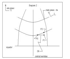
The same types of consequences happen for the UTM plane and the state plane coordinate system when the state plane coordinate system is a Transverse Mercator. Diagram 2 shows the results of laying the Transverse Mercator over the UTM system. The difference in this case is that the offset DX in the horizontal direction results in an apparent rotation in the opposite direction of the rotation in the Lambert conic projection.
FINAL ANALYSIS
It was found that for the most part, the data was translated correctly. There was a small error introduced during conversion that varied from 1-8m, depending on where in the system the data was located. This is considered acceptable since the source data had contained larger errors. The relative distances between items in an area have a negligible error.
Once an understanding of the situation was accomplished, the company could then move ahead with confidence. The importing and exporting of data will happen correctly and the use of GPS is possible. Modifications to the grids used for producing the maps will be made and no further action needs to be taken.
CONCLUSION
It is understood that whenever one portrays a 3 dimensional object on a 2 dimensional surface (paper map or computer screen), some distortion of the image will occur. An appropriate projection system is chosen to meet the need of a given purpose. For the most part, once this decision has been made, one must live within those constraints.
Care must be taken when combining data from different projections systems or in comparing data from different projection systems. When taking measurements or doing calculations, do not mix “units” but keep everything on the same basis. For example, when comparing data from a UTM system to a State Plane system, convert the data of interest to one or the other. After all are in the same environment, then do the comparisons. If you don’t, you open yourself up to the possibility of error and confusion.
Frank B. Weiss P.E.
Principal Consultant
KEMA Consulting