Wetlands have become rare in the European community due to desiccation. These are often strongly influenced by ground water abstraction and drainage of their surroundings. Predicting the effects of water management measures on wet terrestrial ecosystems is an essential element in environmental impact assessment. Knowledge about steering natural processes is used in the expert system NICHE® (Nature Impact Assessment of Changes in Hydro-Ecological Systems). Based on several practical applications, the main concepts behind NICHE® and how it is implemented in GIS are described.
Kiwa Research and Consultancy is the knowledge center for drinking water and associated ecological and environmental questions in The Netherlands. Kiwa is responsible for scheduling and conducting the joint research for Dutch water companies. Over the past 30 years expertise has been built up in diverse areas including hydrology, ecology, process technology and distribution technology. Since 1989 also GIS-technology has been used to support our core competence: the integration of these various fields of knowledge to develop innovative tools and concepts for adequate support of our customers.
Plant communities of wet and moist terrestrial ecosystems ('wetlands') have become rare in the European Community. The deterioration of these wetlands is mainly due to desiccation and still proceeds as the sites are often strongly affected by ground water abstraction and drainage of their surroundings. To prevent further deterioration and to restore the natural environment and related biodiversity, nature conservation and restoration of wet and moist terrestrial ecosystems has become an important aspect of the water management policy of the European Community. Predicting the effects of water management measures on wet and moist terrestrial ecosystems is an essential element in environmental impact assessment studies. Nowadays, governmental organizations, water utility companies and water authorities throughout Europe need instruments that can predict the effects of their activities on the natural environment and give information about measures that may compensate or mitigate for the negative effects of their activities.
Over the Past decades, scientists have developed a high standard of experience in water management and ecological impact assessment. This knowledge can be used in expert systems for making predictions of the impacts of planned measures/activities on water-dependent ecosystems.
An example of such an expert system is the model NICHE® (Nature Impact assessment of Changes in Hydro-Ecological systems). NICHE® uses easily obtainable GIS-data to predict effects on plant communities caused by changes in hydrology, land use or management.
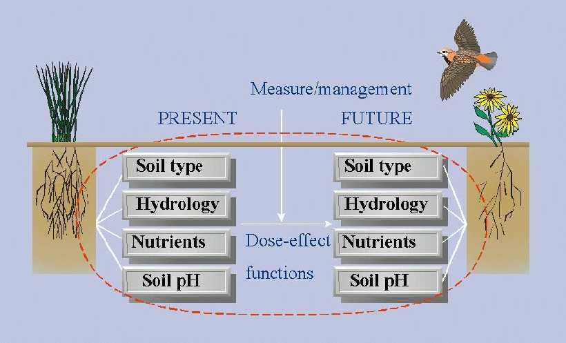
Figure 1 illustrates the ecological concept. NICHE® determines site conditions (nutrients availability, pH ,ground water level) using dose-effect functions. These functions are based on field observations and expert judgement. Predicted site conditions are compared with a database that contains site requirements of plant communities. If predicted site conditions fall outside the range of site requirements for the current vegetation, it is expected that the vegetation will be replaced by vegetation that is adapted to the predicted site conditions.
To enable the comparison of different measures or scenarios, effects are also expressed in 'nature value scores'. Nature value scores are a function of the nature value of the plant community involved and the area that is affected.
Examples of questions that can be answered using the output of NICHE® are:
The following paragraphs will focus more on the technical implementation of the model in GIS.
NICHE® was implemented in 1996/1997 in ArcInfo using a set of AML's and related INFO tables. As such the model is completely embedded in GIS (Heinzer et.al. 1999). For the GIS applications developer at that time it was a huge task to formalize all the necessary expert knowledge. An important choice was made at that time to work with vector processing only, no GRID functions were used. The main considerations were that even very small polygons in the input coverages and overlays needed to be retained in the model output.
Each scenario runs separately through the model. Scenario output comparison is not part of NICHE® itself but has to be done in the postprocessing phase by the user. Most of the pre- and postprocessing is done with ArcView GIS.
Calibration of the model is done manually by comparing the output with current vegetation patterns and field knowledge. Scenarios are developed and translated into changes in model input. These changes may apply to ground water levels and vertical ground water fluxes (seepage / infiltration) calculated by a hydrological model (e.g. Modflow, Microfem). Other scenarios may include alterations in land-use (e.g. from agricultural to nature areas) or land management (fertilization, mowing, sod-cutting, cattle grazing).
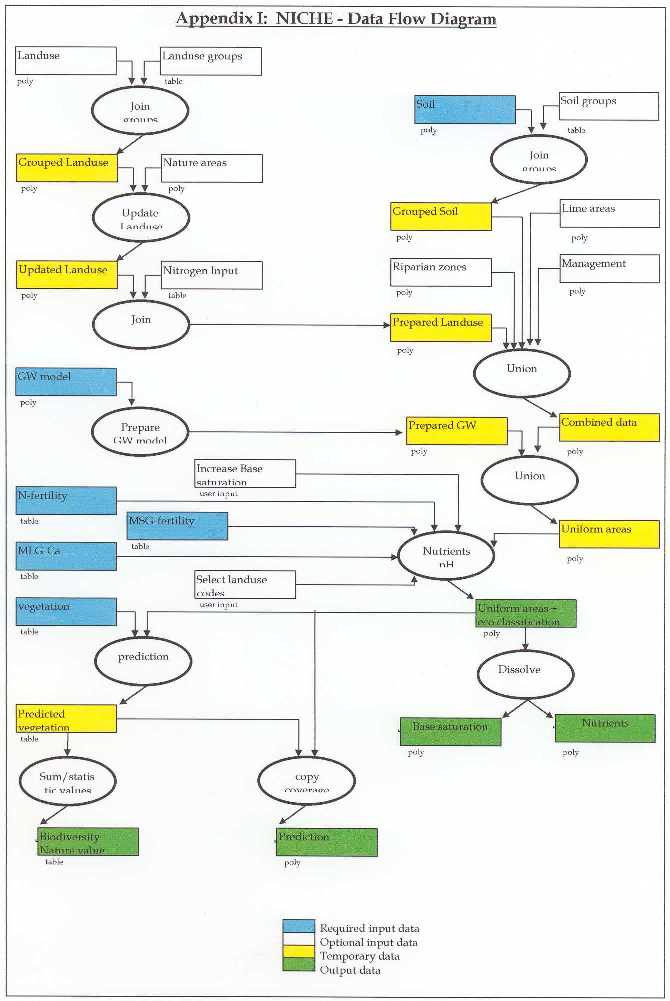
The model consists of 2 mayor parts, the abiotic site characterization and the biotic site characterization (the vegetation prediction). The general structure is illustrated in figure 2. Appendix I provides a more detailed data flow diagram for further reference. Both parts are discussed more elaborately in terms of data input, GIS analysis and data output in the following paragraphs.
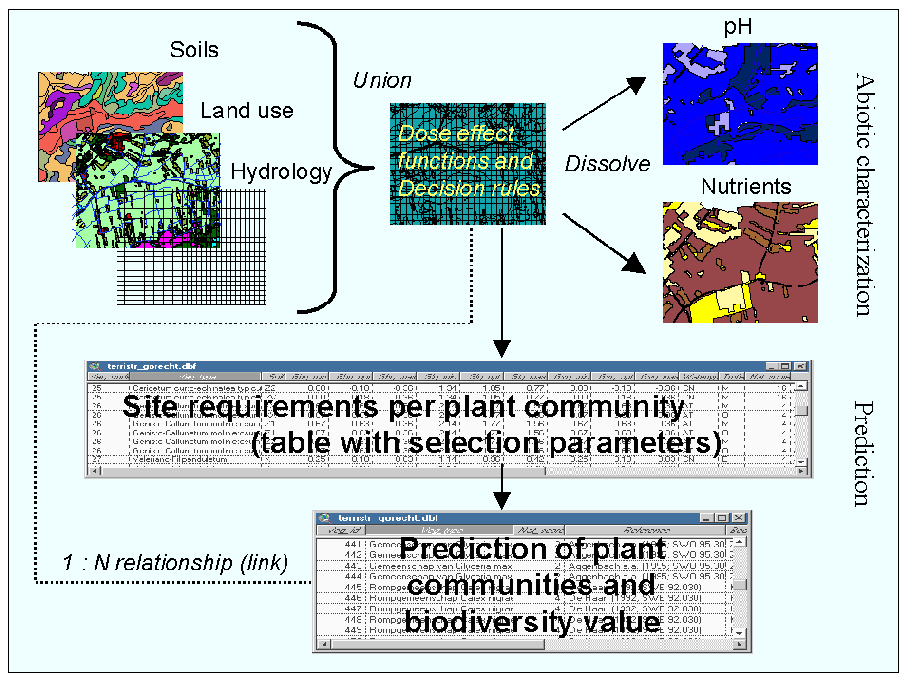
The abiotic state is derived from soil type, land use, hydrology and other optional input data (see appendix I) and using dose-effect functions and decision rules.
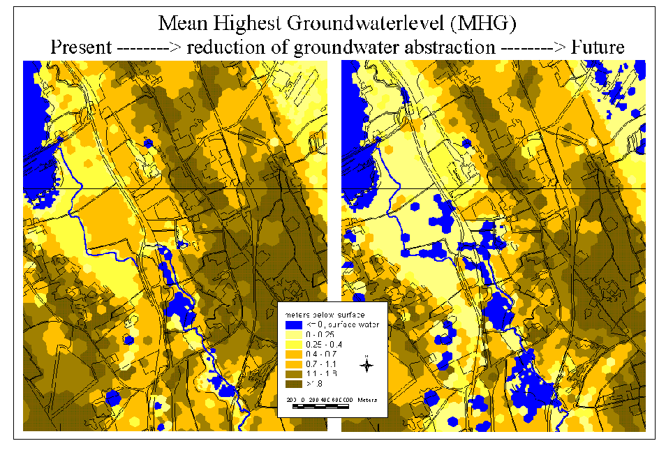
Our main goal with the development of NICHE® was that the model should be applicable for most, if not all, areas with ground water dependent vegetation in the Netherlands. Therefore we have chosen to use easy obtainable data including nationwide polygon coverages of soil units (1 to 50.0000 scale) and 30x30 m Land use grid polygons(based on Landsat imagery) as the standard input for any study area. A typical study area covers approximately 30 km2, for example around a ground water abstraction. A hydrological model is developed to calculate the effects of (changes in) ground water abstraction. The model polygons or nodes are converted to an ArcInfo polygon coverage. If nodes are used Thiessen polygons are created to obtain a polygon coverage of the related values, figure 3 shows an example of this. Sometimes translation and/or rotation of the ground water model is necessary. In most cases a dynamic ground water model is required, revealing estimations of mean phreatic ground water levels in the wet season (Mean highest ground water level - MHG), the growing season (Mean spring ground water level - MSG) and in dry season ( Mean lowest ground water level - MLG). All these values are used to predict nutrient-availability and base-saturation, because they influence the abiotic soil processes (N-mineralization, pH buffering).
Optional input to NICHE® includes; riparian zones (polygons); Nitrogen deposition values (atmospheric, manure and fertilizer) linked to specific land-use categories; ground water flux-type, base-rich (deep ground water) or base-poor (shallow ground water).
The output consists of a polygon coverage with related attribute tables (Info files). This coverage is the result of a number of union, dissolve and clip operations. The soil unit map for example is first grouped in ecological soil units and aggregated by a dissolve operation before a union is made with the ground water model coverage (see appendix 1). The results of every step in the process (decision rules, relationships) are recorded in the attribute table of the output coverage.
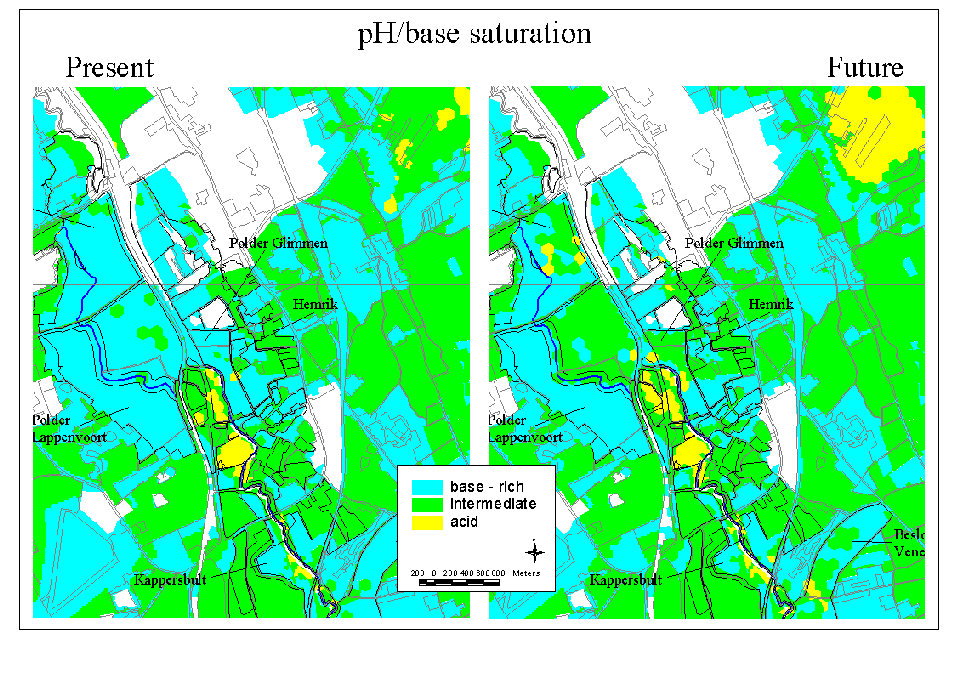
For practical reasons the output polygon coverage is dissolved on the items "Nutrient availability"and "pH/base saturation" (see figure 4). These 2 maps can be regarded as separate model output and play an important role during the calibration phase.
The abiotic characterization of the study area forms the basis for the prediction of ground water dependent vegetation. In the past 10 years we have developed an extensive database on the occurrence of 100 different ground water-dependent plant communities under various abiotic site conditions. This database is used to set selection criteria and predict the occurrence of the plant communities.
Besides nutrient availability and pH/base saturation the soilgroups and ground water levels are also used in the prediction. Plant communities have specific ranges and optima for MLG, MSG and MHG.
Per polygon more than 1 plant community may be predicted because the abiotic ranges of these plant communities may overlap. These predictions are stored in a separate table. When reviewing the output of a NICHE® run a link between this table and the output coverage needs to be established. Now selections per predicted plant community could be visualized.
Each plant community may also have a 'nature-value' score and these scores are also calculated for each polygon in the output coverage. If more than 1 plant community is predicted the nature value score is the mean of the individual scores.
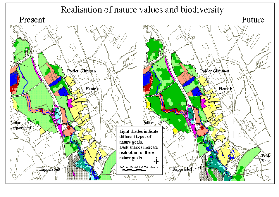
Figure 5 shows yet another way to present the output. Here nature-goals in terms of different groups of plant communities are compared with NICHE® predictions.
After input preparation the user has to set a number of variables in a STARTNICHE.AML (see Appendix II) to start the NICHE® run. Some of these variables serve as ON/OFF switches for optional input. Look at the following few lines from a typical STARTNICHE.AML:
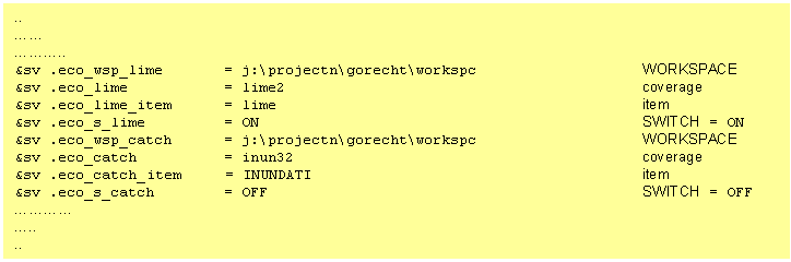
The *catch* variables are set to represent the riparian zones in the area. In this scenario they are not accounted for because the switch = OFF. The *lime* variable is ON and used to indicate areas where lime is distributed to lower the pH and increase the buffering capacity of the soil.
Each scenario has its own STARTNICHE.AML and they are renamed according to the scenario.The appropriate AML is started from the ARC command window, it sets the variables and then it runs NICHE.AML . This main AML prepares the input coverages and tables for further processing. The original data is copied to temporary coverages and tables so the original data is not affected. NICHE.AML subsequently calls a number of submodules stored in separate AML scripts:
A BAILOUT routine is part of all these AML's. In case of an error, the (sub)module is terminated.
A typical NICHE® run processes 50.000 polygons in approximately 1 hour (Windows NT on a Pentium III, 600 MHz, 256 Mb RAM)
A number of limitations of NICHE® are caused by the rigidity of the dose-effect functions and decision rules (of type "if …then… else…") and to the fact that the output is limited to plant communities. Besides this the translation of abiotic site characterization into the prediction of a certain plant community is often based on a limited dataset about this particular plant community . NICHE® does not handle 'uncertainty'. Boundaries between soil units for example are handled as being crisp, not fuzzy. A plant community is either predicted or not, no probability of occurrence is determined.
On the technical level the current NICHE® lacks a module for 'scenario management'. The settings for a NICHE® run are only stored in the STARTNICHE.AML. Several scenarios may use the same coverages and tables with the same (or other) attributes. Sometimes different versions of ground water model coverages are used in the scenarios. A logbook is kept for each project. The user has to maintain the 'link' between logbook, AML's and file structures on the network drives. It is obvious that this link is very weak. It does not necessarily guarantee that model results can be reproduced after a few years although we have to guarantee this for a period of 5 years after completion of the project.
Tracing program execution errors can be a considerable problem at this moment. AML programming does not offer detailed error handling. When starting up a new project it can take several attempts before a NICHE® run is succesfull due to all kinds of 'hidden' input restrictions which have not been encountered previously. Recently we have experienced an increase of these problems because we have started to apply NICHE® in other countries (mainly in Belgium) as well. In these cases not only the vegetation database needs to be updated but also relational tables for soil and land use grouping have to be adapted to local typologies. Therefore implementing the model in another organization (an important part of our activities) may prove to be a difficult process.
Postprocessing of the results may take considerable effort. The questions to be answered are often on a different abstraction level than the output of the model. So the output needs to be selected and grouped based on specific demands.
Together with the Dutch watercompanies we have sought cooperation with several experts at other institutes (the University of Wageningen, the Flemmish Institute of Nature Conservation in Brussels) to think about or comment on some proposed conceptual improvements to the model. Some of the ideas are mentioned here.
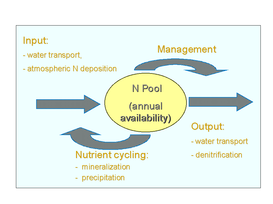
NICHE® produces a static prediction of the vegetation in a presumed stable end-situation . In reality this is a complex dynamic process of vegetation succession stadia closely related to organic matter content of the soil and therefore nutrient availability, pH/base saturation and soil moisture content. In order to provide better predictions there is a clear need to develop and incorporate dynamic soil and nutrient models into NICHE® (see figure 6).
Current ecohydrological research at Kiwa and the Technical University of Delft also focuses on finding a better way to relate ground waterlevels to vegetation. Instead of taking long-term averages of highest, lowest and spring ground water levels more detailed time-series analysis will provide better information on these relationships.
Several experts have pointed out the need for a database with vegetation/species site descriptions linked to field measurements of abiotic parameters. This database must be updated on a regular basis with new field data and will serve as a region-specific datasource for each prediction. The user must have the ability to set a 'search-radius' and other criteria to select the most relevant records from the database in the vicinity of the studysite. New regression techniques can be used to derive functions with confidence limits. These functions describe the relationships between the measured abiotic parameters and abundance of species and/or plant communities. These relationships are then used in site specific decision-rules.
Without doubt we are facing a great challenge to put the new concepts in a new user-friendly software application based on ArcGIS. We want to give the user more control over the model by making it more interactive and dynamic. The user should be able to define measures (like changing ground water levels) and immediately see the results in the abiotic characterization. There should also be an option to enter a vegetation map of the current situation as a starting point for a vegetation prediction of a chosen year after the measure and using the prediction again as a new starting point. A special challenge is to directly incorporate a hydrological model. We have already realized such a prototype with our ArcView-Matlab interface (Raterman et.al. 2001). We expect that interacting with such a dynamic modeling tool will facilitate a more creative process of scenario development.
We have to scrutinize Esri's Component Object Model (COM) and let it interact with other objects (in DLL's). A DLL might serve a hydrological calculation or regression module for example. The Geodatabase may be used to store vegetation survey data and related field measurements of abiotic parameters. Versioning of the geodatabase offers possibilities to model history (see Esri technical paper on this subject) and better scenario management. With raster processing we can build faster modules for abiotic characterization and handle uncertainty as well.
A number of questions arise about whether and how to use the new technology that Esri offers. For example: Is it feasible(technically and financially) to use the Geodatabase and versioning option to better support scenario management if at the same time we want to use rasters for faster calculation?
At the moment several experts still work independently on different modules producing well documented prototypes in their favorite programming environment. This may be either in Fortran, Matlab or C++ code. Using small examples we are currently developping guidelines for them so it will be easier for programmers to create ActiveX DLL's from those prototypes to be incorporated into a new NICHE® based on ArcGIS. During this stage of development it is very important to keep the experts informed about the new possibilities ArcGIS has to offer.
To prevent further deterioration and to restore the natural environment and related biodiversity, nature conservation and restoration of wet and moist terrestrial ecosystems has become an important aspect of the water management policy of the European Community.
The model NICHE® (Nature Impact assessment of Changes in Hydro-Ecological systems) uses easily obtainable GIS-data to predict effects on plant communities caused by changes in hydrology, land use or management.
Data pre- and postprocessing and scenario management may take considerable effort. NICHE® is programmed in AML and does not have a user-friendly interface. Implementation of the model in other organizations can be difficult.
In the near future new ecological and hydrological insights and concepts need to be incorporated into a new more dynamic and user-friendly version of NICHE®.
ArcGIS supports modern techniques for software integration and database management. These techniques need to be evaluated thoroughly before they can be used in a new version of the model.
A typical STARTNICHE.AML
Heinzer, T.J., M. Sebhat and B. Feinberg. 1999. Integrating Geographic Information Systems to Hydraulic Models: Methods and Case Studies. Esri User conference proceedings 1999.
Raterman, B.W., M. Griffioen and F. Schaars. 2001. GIS and MATLAB integrated for ground water modeling. Esri User conference proceedings 2001.
Esri. 2002. Modeling and using history in ArcGIS. Esri Technical paper
Martin de Haan
Arthur Meuleman