Various techniques are presented for integrating GIS with hydraulic modeling of the Lower Colorado River by the US Bureau of Reclamation and Colorado State University. The model is geared towards creating a better understanding of the environmental impacts of dam operations and river control on the critical habitat of endangered species. GIS techniques which are explored include geostatistical analysis of existing data to produce terrain surfaces for use with the model, as well as methods to create high quality visually-oriented representations of model output, including two and three dimensional animations.
The Lower Colorado River (LCR) flows from its division point with the Upper Colorado at Lee’s Ferry, AZ, to its mouth at the Pacific Ocean in Baja California, Mexico. It is currently under the control of eight dams. Prior to the closure of the dams on the LCR, the river was heavily silt-laden, and transported over 150 million tons of sediment annually. It now carries only a fraction of that, and the channel has undergone high levels of degradation (Fagot, 2001; Saiki et al., 1980). The channel bed was once composed of shifting sand, but due to the entrapment of sediment within the reservoirs, the channel has undergone an armoring process, resulting in a bed composition of coarse materials such as gravels, cobbles, and boulders along many lengthy reaches (U.S. Bureau of Reclamation, 1996). The main channel of the river has been straightened and stabilized in most areas to control flooding, resulting in the loss of most in-stream spawning sites and some pond areas separated from the main channel, also known as backwater areas. Flows in the river once fluctuated greatly, resulting in a harsh environment that was only inhabited by eight species of freshwater fish. After the completion of Hoover Dam in 1935, the flowrates within the river became much less variable. The increased stability has allowed non-native species to flourish, and today most of the fish found in the LCR are non-native (Minckley, 1979; Saiki et al., 1980). Many of these are predators to the native species. Of the native species, two of particular interest have been listed as endangered. These are the Razorback Sucker and the Bonytail Chub.
It is highly uncertain what physical changes will provide proper breeding and rearing habitat for native species, however due to the social and political problems associated with altering the present main channel stability, the current approach focuses on the backwater ponds which are separated from the channel. Prior to the creation of reservoirs on the LCR, the number and size of backwaters along the river were limited due to high evaporation rates and siltation. These backwaters were clearwater areas which generally became a part of the main channel area during periods of high flow. Subsequent to dam closures along the river, many of the backwaters became permanent, and some were lost due to lowered water tables. Early attempts to mitigate the loss of sport fishery involved the creation and maintenance of many shallow backwaters through dredging. Additionally, channels or culverts were constructed to keep backwaters connected to the main channel of the river (Saiki et al., 1980).
The environmental, ecological, engineering, and biological communities have expressed concern over the effects of river and reservoir operations on the habitat in these backwater areas. Engineers from the Bureau of Reclamation, in conjunction with Colorado State University, are utilizing hydraulic models to assess these effects. The models predict the water surface elevations within the backwaters during the passing of a hydrograph created by dam releases and river operations. By analyzing and studying the change in water surface elevation, an attempt can be made to determine the change in habitat for many species of life living in the areas. Analysis and visual support for the models have been provided through the use of a geographic information system (GIS). The GIS is used to provide valuable input data for the hydraulic modeling portion of the study, and a tool has been created to produce an analysis and visualization of the output from the model. The visualization serves to graphically illustrate the effects of various river operations on the habitat in the backwaters.
Proper hydraulic modeling of the backwaters requires high resolution bathymetric data for the backwaters. Additionally, this data is important for the analysis of the model output. Three types of data were available for this study. Though each type of data has is own merit, none of the data was directly useable for the modeling of the river. Limitations on each of the different types of data precluded them from direct use. These types of data and their limitations are outlined as follows:
Illustrations of the three types of available data are shown in figures 1 and 2.
Figure 1. - Bathymetric survey transects and infrared water edge boundary
Figure 2. - 3D view of USGS 30m DEM.
To produce a suitable bathymetric surface for the hydraulic modeling, geostatistical analysis was used. The bathymetric data was combined with the water edge data to produce a dataset of points representing known elevation values in the backwater. This dataset was then processed using the Geostatistical Analyst © extension to Esri's ArcGIS © software to produce a statistically estimated bathymetric surface. USGS DEM values were used to provide an estimate of the terrain surrounding the backwater. The ordinary kriging method of analysis produced bathymetric surfaces which were acceptable for use in the hydraulic modeling effort. It is important to note, however, that the surfaces represent an estimate of the actual terrain, and cannot replace a thorough survey for proper modeling and analysis. A set of combined data points and their corresponding geostatistical surface are illustrated in Figure 3.
Figure 3. - Combined set of data points and their corresponding geostatistically generated surface.
To assist the hydraulic modeler in the creation and setup of the model, a visual tool for data storage was needed. One of the goals of the effort was to provide a view of the river itself in relation to the locations of river survey data, such as river cross-sectional data and backwater data. Using the tool, the modeler would be able to make better decisions while creating and calibrating the model. Another goal of the visual data storage tool was to reduce model setup time and cost. It was decided that the tool should operate from a web browser, to allow use on all systems and platforms.
To provide a cost effective solution while avoiding many known problems with existing products, a new application was created using Esri’s Avenue © scripting language for the ArcView 3.x line of products. This application allows the user to create an interactive web site which displays specified geographic layers. The application also provides the user with the ability to create hypertext links on the site for selected features in a geographic layer. These links open new browser windows that display any type of predefined information such as data, feature attributes, images, animations, etc. In this manner, the user of the application can display pertinent data for hydraulic river modeling, such as a plan view of the river itself, in relation to input data for the model. This input data would include river cross-sectional data and elevation-capacity curves for backwater areas. The tool is illustrated in Figure 4.
Figure 4. - Visual data tool, with pan, zoom, and select capabilities.
Three distinct types of programming code are utilized in the application. A flow chart of the application operation is shown in Figure 5. User specified layers are processed within ArcView using an Avenue script to create a set of static JPEG images, as well as a PERL coded text file. The images and text file are then transferred to a web server where a PERL compiler has been installed. When a web browser interfaces with the PERL file, parameters are passed to the code that specify properties such as location, zoom level, and selection mode. Operating on these parameters, the PERL code presents the web browser with a properly formatted HTML page containing the user requested map. Whenever the user interacts with the map from the browser, a new set of parameters is passed to the PERL program, resulting in a new map. The maps presented in the web browser can optionally have features that are linked to other web pages. In this manner, the user can select a desired feature (such as a surveyed river cross-section or backwater) and display pre-defined information about the feature. Assuming the feature includes input data for the hydraulic model, the user may directly enter the data into the model by copying the data from the browser window, thus accelerating model setup while providing a visualization of the river being modeled.
Figure 5. - Flow chart of web application operation
Backwater areas along the river are of particular interest due to their suitability as habitat for many species of animals. Of particular interest are two endangered species of fish in the LCR, the Razorback Sucker and the Bonytail Chub. Additionally, one species of endangered bird, the Southwestern Willow Flycatcher, is believed to nest in areas adjacent to the backwaters. The GIS can be used to analyze the changes in habitat in the backwater areas, based on historic river flows or the output from the hydraulic model.
To analyze and visualize the changes in the backwaters, a GIS tool was created. Provided a time series of water surface elevations in a backwater area, the tool calculates the following values:
These calculations can be analyzed to provide a variety of results. These results may show such statistics as the amount of surface area for all depth intervals at a particular time step, or the change in surface area associated with a particular depth range throughout a particular period of time. Additionally the tool can provide the following types of animation:
These animations can have any background for the surrounding terrain, including aerial/satellite photography, topographic maps, land use / land cover mapping, etc.
The tool was written in Microsoft's Visual Basic © programming language as a custom dynamic link library (dll). The dll is opened in Esri's ArcMap © or ArcScene ©. When opened in ArcMap, the dll creates a toolbar which provides the user with a combo box displaying all available raster layers in the document. The user selects a raster layer representing the backwater terrain, such as one of the geostatistically created backwater bathymetry layers. The user then enters an "analysis interval" value into a text box on the toolbar. This number specifies the interval that defines the ranges in depth which will be analyzed (e.g. for an interval of 1 ft, ranges of 1-2 ft, 2-3 ft, 3-4 ft, etc.). The user can optionally enter the limits of a "critical depth range" or range of depths for a focused analysis into text boxes on the toolbar. The user then selects either the "Analyze Backwater..." command or the "Visualize Backwater (2D)..." command. Depending on the command selected, the user will be prompted for a file of time-series water surface elevation values, and a filename for the output analysis file or animation file. When opened in ArcScene, the toolbar provides similar functionality, however the only command available is "Visualize Backwater (3D)...". The toolbar is illustrated in Figure 6.
Figure 6. - Custom toolbar for analysis and visualization.
Depending on the command selected, the tool creates a text file of analysis values for further study, or a Video for Windows (avi) formatted file which illustrates the change of the water surface in the backwater over time. In this way, the user can analyze the changes in habitat within the backwater, numerically or visually. A single frame of a 3D animation is shown in Figure 7.
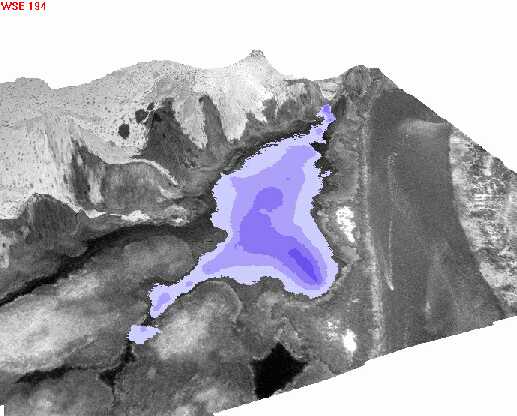
Figure 7. - Single frame of an animation showing the water surface in a backwater pond.
Fagot, Kevin, 2001. Endangered Species Along the Lower Colorado River. In: D.F. Hayes (Editor), Designing Successful Stream and Wetland Restoration Projects; Proceedings of the 2001 Wetlands Engineering and River Restoration Conference. ASCE, Reno, NV.
Minckley, W. L., 1979. Aquatic Habitats and Fishes of the Lower Colorado River, Southwestern United States : Final Report. U.S. Bureau of Reclamation, Lower Colorado Region, Boulder City, NV.
Saiki, Michael K., Kennedy, David M. and Tash, Jerry C., 1980. Effects of Water Developments on the Lower Colorado River. Cal-Nevada Wildlife Transactions: 100-111.
U.S. Bureau of Reclamation, Lower Colorado Region, 1996. Description and Assessment of Operations, Maintenance, and Sensitive Species of the Lower Colorado River : Biological Assessment. U.S. Bureau of Reclamation, Boulder City, NV.