Advances in DNA sequencing have resulted in data generation that has far outpaced the available visualization and analysis tools needed for efficient interpretation of these data. In order to understand the biological significance and interconnectedness of these data, we have developed GenoSIS (Genome Spatial Information System) as an application of the concepts and tools of geographic and spatial information science to the interpretation and modeling of genome data. Our implementation of “spatial genomics,” which uses Esri ArcGIS and Oracle Spatial, allows us to reuse existing spatial analysis, classification, querying, and visualization tools for genome data analysis.
The primary motivation for developing GenoSIS is to support the use of sequence feature maps as tools for pattern discovery as well as graphical abstraction of genome content. It is our assumption that, in addition to having a “parts list” of an organism’s genome, researchers want to explore potential biological significance in how genome features are organized. The visualization component of GenoSIS is more dynamic than genome browsers that are “display only.” For example, GenoSIS allows users to create attribute choropleth maps on the fly in response to such simple queries as “Draw a sequence feature map in which all genome features that are annotated as being involved in DNA replication are displayed in blue.” By integrating pattern detection and pattern matching methods directly with genome visualization, GenoSIS can be used as a tool for generating hypotheses about the biological significance of genome feature organization.
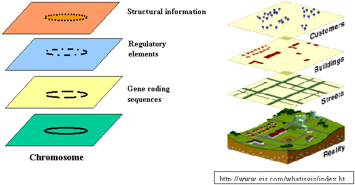
The layered map, a concept fundamental to GIS, provides a useful approach for the integration of diverse biological data: DNA and protein sequence data, gene functionality data, biochemical pathways data, and even image data can be coordinated by location in the genome as different layers of a single genome map. One can mix and match queries, analysis, and visualization among and within layers.
The particular advantages to representing genome
data in an already developed spatial information system like ArcView (Esri,
2001) integrated with the Oracle Spatial database (Oracle Technology Network,
2001) include:
· Powerful standard built-in GIS visualization, query, and analysis tools;
· Facility to incorporate additional customized tools for spatial data analysis or other functions in the GIS user interface;
· Availability, as part of the database, of spatial functions, which are of special use to express the complex interrelationships of genome features.
The combination of these features makes for a very powerful analytical tool. Functionally, GenoSIS allows users to view sequence feature maps as graphical objects at user defined scales of resolution. Query generation and response is tightly integrated with the visualization component of the system. Multiple scales allow for detection of patterns that might be scale-dependent. If a significant pattern is detected, a user has the ability to test the statistical significance of the pattern and also to use the pattern as a query to search for it in another genome.
“It now is commonplace to describe molecular biology as being in the middle of an information explosion...this explosion of information is changing the way science is conducted in the field of molecular biology...” (Collado-Vides, 1996). “An unprecedented wealth of data is being generated by genome-sequencing projects and other experimental efforts to determine the structure and function of biological molecules. The demands and opportunities for interpreting these data are expanding more than ever.” (Baldi, 1998)
An organism’s genome is the full complement of its DNA, which is organized as one or more chromosomes. Arranged along each chromosome in a linear order are thousands of genome features of biological significance that have been annotated by molecular geneticists. These features include genes and the regulatory elements that control expression of genes.
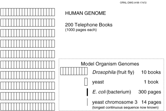
In the last few decades, advances in molecular biology and the equipment available for research in this field have allowed the increasingly rapid sequencing of the genomes of many species and, currently, the whole genomes of some 800 organisms is available. GenBank (Benson, 2000) is a widely used repository of DNA sequence information. As of April 2002, there are approximately 19,073,000,000 bases in 16,770,000 sequence records in GenBank, and the resource is growing exponentially ( http://www.ncbi.nlm.nih.gov/Genbank/GenbankOverview.html ). The figure below from the Oak Ridge National Laboratory Primer on Molecular Genetics (http://www.ornl.gov/hgmis/publicat/primer/toc.html ) gives a sense of the amount of information in the human genome.
This huge amount of information has necessitated the
application of the methods of information science to biology giving rise to
the fields of bioinformatics, genomics, and computational biology. While the
problem of storage and organization of ever increasingly complex data and
providing access to it through researcher-friendly interfaces is itself a
challenge, the most pressing tasks in bioinformatics involve extracting knowledge
from the data through analysis such as recognizing genes and other features
in sequence information, predicting structure and function of proteins, understanding
protein interactions in biochemical pathways, and relating similar proteins
in different organisms as a way of examining evolutionary relationships among
organisms.
There are many cases where the spatial organization of genome features has been shown to have biological significance. Recent studies related to gene finding and genome annotation (Rogic et al., 2001), provide evidence of complex spatial interrelationships of genome features: genes are alternatively spliced, genes may be nested within other genes, and genes may overlap. Conservation of gene order in microbes has been a subject of a great deal of analysis (Tamames, 2001).
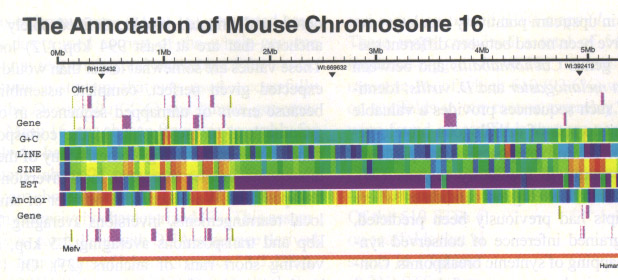
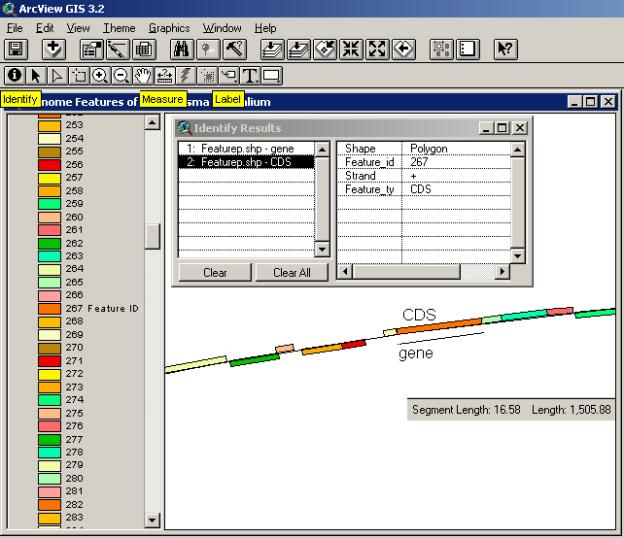
The draft assembly of the mouse genome has just recently been made public ( http://www.sanger.ac.uk/Info/Press/020506.shtml ) and annotation of one particular mouse chromosome (Mural, 2002) seems to indicate that humans and mice share about 97.5 per cent of their working DNA. The arrangement of a number of genome features is shown in the chromosome segment below. Color-coding of different non-spatial attributes of the features and side-by-side alignment are used to illustrate the annotation.
This level of human-mouse similarity is somewhat surprising since this is just one percent less than the amount shared by humans and chimpanzees. Previous estimates had been that humans and mice would differ by as much as 15 percent. In all likelihood this conservation is the result of preserving essential functions from the two species’ common ancestor 100 million years ago until today. But, in addition, the researchers speculate that the genes might actually all be identical and that the differences between the species may be due to differences in the regulatory elements that control the expression of the genes. It is well known, for example, that certain regulatory elements have spatial dependencies relative to transcriptional start sites of genes.
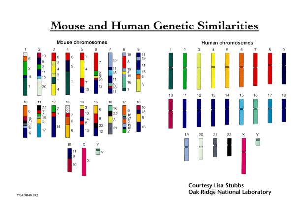
Previous work has shown that the genetic similarity of the superficially dissimilar mouse and human species is such that the human chromosomes can be cut up into some 150 segments and reassembled to a close approximation of the mouse genome as shown below.
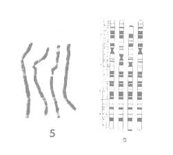
The figures above are taken from an article (Yunis, 1982) comparing the chromosomes of human, gorilla, chimpanzee, and orangutan. The figure on the left shows a chromosome 5 image of the four species placed side by side. Depending on chromosome structure and biochemical composition, a chromosome shows distinct patterns of segments or bands of light and dark staining, when treated with a dye and observed under a microscope. The corresponding figure on the right shows a cytogenetic map, a stylized map of the chromosomes indicating the characteristic bands. The map clearly shows regions of significant similarity or homology as well as regions of significant difference among species.
Another type of map used by geneticists, the genetic-linkage map, was developed in 1913, before scientists knew that genes were made of DNA, to study the spatial association of genes in fruit flies. Rather that actual location along the chromosome, the linkage map shows the relative position of genes based on the rate at which two different genes are inherited together or separately in genetic studies.
With the advent of methods for sequencing DNA and manipulating cloned DNA, it is now possible, in principle, to produce a physical map, which associates a precise position on the chromosome with each gene. Additional methods allow genome cartographers to combine the landmarks of these various maps as shown below in order to take advantage of the best features of each type of map. The chromosomal and linkage maps show an entire chromosome with corresponding positions connected by lines; the physical maps, measured in kilobases (kb) show a detailed view of a portion of the chromosome with the last map indicating a single gene with more detail of structure visible at this scale.
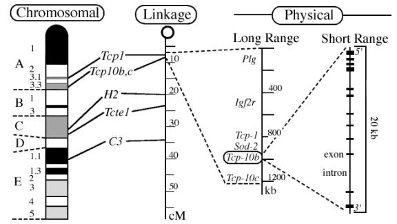
http://www.informatics.jax.org/silver/frame1.3.shtml
(Silver, 1995)
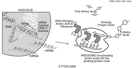
The figure below (Casey, 1992) is a representation
of the process we are concerned with in the current version of GenoSIS:
In the nucleus of a cell a segment of DNA that is a gene is copied (transcribed)
to messenger RNA (mRNA) which is transported to another part of the cell,
the ribosome, in which the mRNA is translated to a chain of amino acids
which will become a protein. Each protein performs a certain role in the
cell usually interacting with other proteins in a series of complex biochemical
pathways. Functionally, at the least detailed level of our system is the
particular organism, which has one or more genomes, which has one or more
chromosomes, which has numerous features. Both chromosomes and features
are DNA sequences, at the most detailed level of resolution we provide the
user access to the sequence information. Since features may be composite,
for example, in some organisms genes are made up of exons (parts that are
translated) and introns (parts that are not translated), we indicate that
a feature may be itself be composed of a set of “subfeatures.”
We began by describing a spatial genomics data model that is intuitive to the biologist querying genome feature information by attempting to make a comprehensive list of features and interactions in the part of the real world of interest for the biologist. This list is the starting point for constructing a list of entities and relationships in our conceptual model. We implemented the data model in an Oracle 8i object-relational database (ORDB). We used several ORDB features to represent complex structured data: user-defined object types, references, and nested tables. The figure below represents the implemented data model, showing how various aspects of the data model correspond to particular facilities of Oracle 8i.
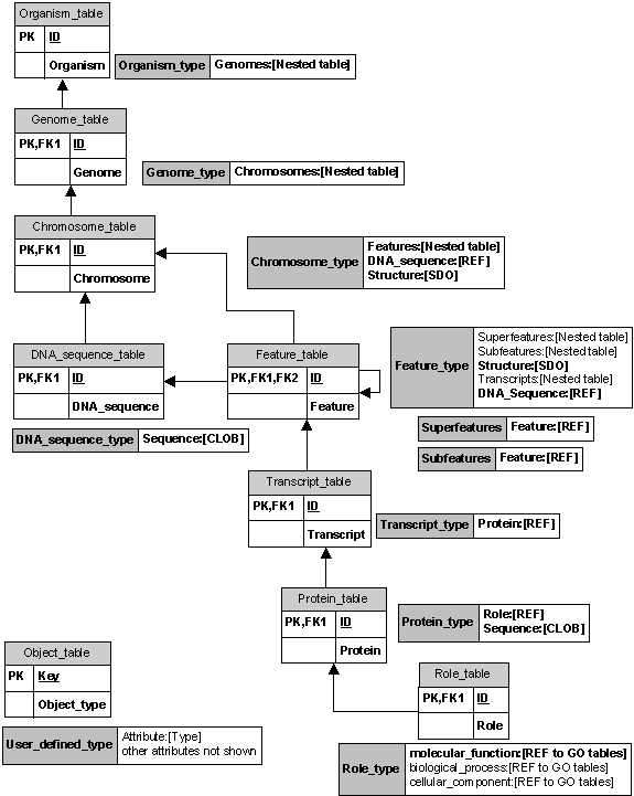
An object-relational database allows for user-defined object types, which makes building the database more intuitive. Object types can be used to map an object data model directly to an object-relational database schema, rather than restructuring the data model into the flattened row-column format of relational tables in a purely relational database. An object-relational database allows for the use of user-defined object types in application programs that access the database, which makes using the database more intuitive. Application programs can retrieve and manipulate the data as objects and call procedures that use the methods of the object type to perform operations on the object. Since the methods can be stored in the database, data-intensive procedures can be more efficient. Objects can be reused, which makes application development faster and more efficient since the use of objects relieves developers of the need to write a mapping layer between application program objects and database objects. The use of objects, based on the underlying software engineering principle of data abstraction and encapsulation, also makes it easier to understand application program code and to maintain application programs.
Each of the objects in our data model is made into an object type: organism, genome, chromosome, DNA sequence, feature, feature set, transcript, protein, and role. The role object points to a set of relational tables representing the current Gene Ontology, which is imported “as is” from the GO site (Gene Ontology, 2000). An object table is built from each of these object types, for example, a table of organisms. Each organism has attributes including an identification number, a genus, a species, and a set of genomes. Most of the organism object attributes are standard SQL data types. The organism type is created with attributes: identification number of number type; genus and species of text string type. But its “genomes” attribute is not a simple value; it is a set of genome objects. We represent the organism’s set of genomes as a nested table, a data structure that is part of the Oracle ORDB system.
A nested table is an unordered set of data elements,
all of the same data type. Nested tables are useful for representing a containment
hierarchy or a one-to-many relationship. In our model an organism stands
in a one-to-many relationship with its genomes. So we represent an organism’s
genomes as a nested object table of genome objects. Similarly, for a genome’s
set of chromosomes, the chromosome’s set of features, and so forth.
The Oracle built-in reference data type (REF) is used
to model many-to-one associations among objects, which reduces the need
for foreign keys and joins. A REF is a logical “pointer” to a row object
and provides an easy mechanism for navigating between objects. For example,
many features are associated with the DNA sequence that corresponds to the
chromosome containing those features, so the feature object contains as one
of its attributes a REF to the corresponding DNA sequence object. In our
model we also use a REF to a role object as an attribute of the protein object
for the one-to-one relationship of protein to role.
Large objects (LOB) are designed to support unstructured data, which tend to be large and cannot be decomposed into standard components. Our model implementation uses character large object (CLOB) type for the nucleotide sequence attribute of DNA sequence object and for the amino acid sequence attribute of protein objects.
Spatial data objects (SDO) are implemented in Oracle Spatial (Oracle Technology Network), which is an integrated set of functions and procedures that enables spatial data to be stored, accessed, and analyzed quickly and efficiently in an Oracle8i database. Spatial data represents the location characteristics of real or conceptual objects as those objects relate to the real or conceptual space in which they exist. Any spatial object will have a spatial attribute, which is the geometric representation of its shape in some coordinate space. This is referred to as its geometry and is a vector-based representation of the shape of the feature, for example, an ordered sequence of vertices that are connected by straight-line segments or circular arcs. Oracle Spatial supports three geometric primitive types: points and point clusters; line strings; n-point polygons and geometries composed of collections of these types.
Spatial objects can be queried through a set of operators and functions for performing area-of-interest and spatial join queries. These methods determine the spatial relationships between entities in the database based on geometric locations, topologies and distances.
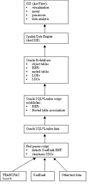
Overall, there are three main implementation
components to the current prototype Genome Spatial Information System architecture
as shown in figure:
· Genome sequence and feature information are extracted from GenBank (and other source) flat text files using a Perl script,
· Sequence feature information and feature attribute data are written to an Oracle object-relational database using a loader utility,
· A GIS graphical user interface, ArcView or ArcGIS, communicates with the database via the ArcSDE (or other) data translator, and allows users to view, edit, and analyze the genome sequence feature maps and takes advantage of tools developed for geographic applications.
· Where is it? How much is there at that location?
· Is there regularity in its distribution? What is the nature of that regularity? Why should the spatial distributional pattern exhibit regularity?
· Is it found throughout the world? Where are its limits? Why do those limits constrain its distribution?
· What else is there spatially associated with that phenomenon? Do these things usually occur together in the same places? Why should they be spatially associated?
· Has it always been there? When did it first emerge or become obvious? How has it changed spatially (through time)?
· What factors have influenced its spread? What geographic factors have constrained its spread?
· Where do we find consensus sequence elements (CSEs)? How many elements are there at that genomic region?A sequence feature map is a one-dimensional, graphical representation of all recognized sequence features. Sequence feature maps are understood to be over-simplifications of what genome space is actually like. Sequence features that appear to be spatially disjunct according to a linear representation of a genome, may actually be close neighbors due to the folding of DNA into a multi-dimensional molecule. As the folding of genomes is better understood, we will incorporate this knowledge into a more complex graphical representation method. In the meantime the simpler one-dimensional sequence feature map representation method will be employed for this project for displaying genome sequence features.
· Is there regularity in their distribution? What is the nature of that regularity? Why should the spatial distributional pattern exhibit regularity?
· Are CSEs found throughout the genome? What are the limits to where they are found? Why do those limits constrain its distribution?
· Are there regulatory elements spatially associated with a gene with a particular molecular function? Do these regulatory elements and genes usually occur together in the same places? Why should they be spatially associated?
· Has a particular gene always been there? In which organism did it first emerge or become obvious? How has it changed spatially (through evolutionary time)?
· What factors have influenced its duplication or deletion in the genome? What factors have constrained its spread?
Baldi, Pierre and Soren Brunak. (1998) Bioinformatics: The Machine Learning Approach, MIT Press, Cambridge.
Benson, D.A., Karsch-Mizrachi, I., Lipman, D.J., Ostell, J., Rapp, B.A. and Wheeler, D.L. (2000) GenBank. Nucleic Acids Res., 28, 15–18. "GenBank" http://www.ncbi.nlm.nih.gov/Genbank/index.html (March 2001).
Casey, Denise. (1992) Primer on Molecular Genetics, Human Genome Management Information System, Oak Ridge National Laboratory, for the 1991-92 DOE Human Genome Program Report. http://www.ornl.gov/TechResources/Human_Genome/publicat/primer/intro.html
Collado-Vides, J. (1996) Integrative Approaches to Molecular Biology , Collado-Vides et al. ed., MIT Press, Cambridge, 179-203.
Esri. (2002) http://www.Esri.com/software/arcgis/index.html
Gene Ontology: tool for the unification of biology. The Gene Ontology Consortium (2000) Nature Genet. 25, 25-29.
Mural, Richard J. et al. (2002) A Comparison of Whole-Genome Shotgun-Derived Mouse Chromosome 16 and the Human Genome. Science, 296, 1661-1671.
Oracle Technology Network. Oracle Spatial User's Guide and Reference. http://technet.oracle.com/doc/oracle8i_816/inter.816/a77132/toc.htm
Rogic, S., Mackworth, A. K. and Ouellette, F. B. (2001). Evaluation of gene-finding programs on mammalian sequences. Genome Res 11(5), 817-32.
Silver, Lee M. (1995). Mouse Genetics Concepts and Applications. Oxford University Press. (Adapted for the Web by: Mouse Genome Informatics,The Jackson Laboratory, 2001)
Slater, F. (1982). Learning through Geography. Heineman Educational Books, Ltd. London, UK.
Tamames, J. (2001). Evolution of gene order conservation in prokaryotes. Genome Biol 2(6).
Yunis, Jorge J. and Prakash, Om. (1982) The Origin of Man: A Chromosomal Pictorial Legacy. Science, 215, 1525-1530.