Lifemapper is a digital library that serves species distribution data on a global scale. Using a distributed Internet query architecture to retrieve georeferences from biological specimen databases in museums worldwide, we create maps and predictive models of species ranges based on environmental correlations with locales where species are known to occur. To parallelize the computation of each independent species prediction we created a screen-saver client that performs predictive analyses on desktop computers before uploading the resulting model to the Lifemapper server (http://Lifemapper.org). Lifemapper uses San DiegoSupercomputer Center's GARP algorithm, Esri’s ArcIMS, ArcSDE and Microsoft’s SQL Server as its primary software components.
Introduction
Conservation and understanding of the earth’s biological diversity is a multi-disciplinary, multi-sector and multi-national activity. Museums around the world have been surveying and cataloging life for the last 250 years, primarily for the purposes of species discovery and description. Non-scientists are largely unaware of vast amount of information represented by an estimated 3 billion museum specimens worldwide, and the geospatial information from the collections themselves have been underutilized beyond the primary cataloging needs of the original collectors. Lifemapper harvests the geographical information associated with specimens and repurposes it as input data for predictive modeling of species distributions. The Lifemapper project aims to highlight the role of biological collections institutions in the documentation of biological diversity by delivering specimen data to the desktops of PC users worldwide. Lifemapper then uses a desktop screen saver to calculate species distribution prediction models. Finally, we archive the models on an Internet server and make them available to the public on the Lifemapper web site (http://Lifemapper.org).
Using the Species Analyst network (Vieglais et al., 1998, http://tsadev.speciesanalyst.net), we regularly query participating museum databases for geospatial information and cache the results. Museums maintain ownership and control locally of their data, but they allow us direct live access to them. The combined specimen data is then analyzed with environmental variables to produce distribution maps for species. It is this analysis that constitutes the bulk of the computing power required. Starting with over one million geo-referenced specimen records and 30,000 unique geo-referenced taxa, the amount of computation required is significant. To scale our computational power to meet the challenge, we followed the ‘embarrassingly’ parallel computation model of the SETI@Home project, which enlisted personal computers to analyze radio signals for indications of extraterrestrial life. In our distributed computing model, users or ”Lifemappers” run a screen saver in the background of their computer that analyzes data downloaded from our server about life on earth. The downloaded data packet consists of museum specimen occurrence points and environmental variables. The screen saver uses an algorithm called GARP, the Genetic Algorithm for Ruleset Prediction, to perform the analysis. GARP is an iterative, non-deterministic algorithm that analyzes the relationships between point locations and environmental variables associated with those locations. The screen saver then returns the data packet to our server for some post-processing, spatial data archiving, and web presentation.
To join the Lifemapper effort, users register and download the screen saver. With registration, Lifemappers can specify preferences, for example, for the class of organism for which they prefer to compute models. Lifemappers can also create and join computing groups. The server tracks computing time and models computed for individual Lifemappers and for groups and presents those statistics on the server.
Methodology
Lifemapper models the correlations between known species locations and environmental variables at those locations to produce species distribution maps. The essential data sets of the project are species occurrences and environmental data sets or layers. Species occurrences are based on point locality data associated with museum specimen records.
The second class of data is a set of global geographic layers corresponding to different environmental parameters, such as temperature, rainfall, tree cover, and others. The layers are stored as grids, where each cell contains the value of an environmental parameter at that location. Lifemapper currently uses about 30 different environmental layers. The University of Maryland provided two variables, percentage of tree cover and land-use/land-cover, at 1 km resolution. The USGS provided terrain data (aspect, flow directions, flow accumulation, slope, and wetness index) at a scale of 1:250,000 that were resampled to 1 km resolution. Climate data was obtained from the Intergovernmental Panel on Climate Change (IPCC) at a resolution of 0.5 degrees, which was then resampled to 1 km to match the other datasets. Climate variables consist of January, July, and year averages for 1961-1990 of cloud cover, diurnal temperature range, ground-frost frequency, maximum, minimum and mean temperature, precipitation, solar radiation, vapor pressure, wet-day frequency, and winds.
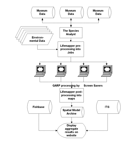
The three stages of data processing for Lifemapper, pre-processing, client processing, and server post-processing, are summarized in Figure 1.
Figure 1: Lifemapper data processing. Server pre-processing consists of data collection via distributed Internet query. Client processing is accomplished with distributed screen saver clients. Server post-processing aggregates, stores and serves the results in an Internet archive of specimen data points and distribution models. The server also combines ancillary species data such as common names from other biodiversity web services.
Server Pre-processing
Pre-processing consists of data preparation. The TaxonSniffer application harvests data from biodiversity databases with the Species Analyst (TSA) architecture then uses ArcObjects to store them in ArcSDE. TSA uses Z39.50 protocol and XML for data retrieval from a network of participating institutions that are accessible over the Internet. A second application, the PreProcessor, combines georeferenced species data points for individual species, calculates the geographic extent of the points, and then prepares a packet of data (a job packet) in XML format for distribution to Lifemapper clients.
Client Processing
The Lifemapper screen saver (Figure 2) implements an evolutionary algorithm called the Genetic Algorithm for Ruleset Prediction (http://biodi.sdsc.edu), or GARP (Stockwell and Peters, 1999). This method has been shown to be the best available method for reliable species predictions using small sets of ad hoc data typically returned from museum databases (Stockwell and Peterson, 2002). The algorithm creates a set of rules to predict presence or absence of a species at a cell, then iteratively tests and modifies them.
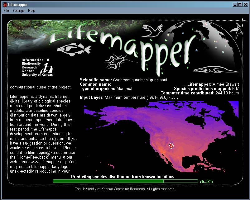
Figure 2. Lifemapper Screen Saver. The screen saver predicts species habitat distribution for a set of occurrence data and environmental layers using the GARP algorithm.
When the screen saver application begins, it requests a job packet from the server. Upon receipt, the application checks the geographic extent of the job packet and, if the environmental data set with the matching extent is not present, it requests that data set. The screen saver processes the job using the data points, the environmental data set, and the GARP algorithm. Once the job is complete, the screen saver submits the job back to the Lifemapper server.
Server Post-processing
After a completed job is submitted to the server, the PostProcessor, an application using ArcObjects and Visual Basic 6, creates a grid by projecting the rules of the model back onto the environmental layers. The application then adds the grid to an aggregate grid for that species and stores it on the file system. A second application, the ModelStorer, converts aggregate grids to vector format and then adds the polygons to a single ArcSDE layer that stores all species models.
Display
The results of the processing pipeline are graphically displayed on the Lifemapper web site (http://www.lifemapper.org) from the Maps and Models menu. The mapping application was created using the ArcIMS, ArcSDE, ArcIMS Active X Connector and VBScript. This application allows the user to query the database for a species by scientific or common name, then map the point locations and aggregate distribution models for each species. Other services provided by this application include opportunities for users: to view current database statistics on points and models for that species, to view points by contributing institution, and to review distribution points or models.
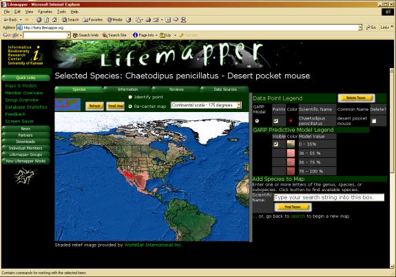
Figure 3. Lifemapper Mapping Application. The Lifemapper map page displays species data points and aggregate distribution models archived archived on the server.
A second graphical application created in compliance with the Open GIS Consortium’s (OGC) Web Mapping Service standard, WMS, is a web service that will return an XML file describing the capabilities of the map service or a map image that can be inserted into another web page. To return the capabilities XML file, a query string (the portion following the ‘?’) must be attached to the base URL (i.e. http://www.lifemapper.org/lm-apps/MapWMS/?Service=WMS&Request=GetCapabilities). There are several required and optional parameters for constructing a map query that are described at the Web Mapping Service under the Downloads menu of the Lifemapper web site. This application was built with ArcIMS Active X Connector and Visual C#.
Discussion
Lifemapper recovers underutilized geospatial data associated with biological collections and brings them into a predictive science framework. By combining museum data with global environmental data layers we are able to predict the present and future spread of species ranges. By changing environmental regimes, such as by applying global climate change scenarios to baseline environmental coverages, we can predict the influence of changes in temperature and rainfall on the distribution of species. By bringing the results of these simulations to an open-access web server and web mapping service, we can promote a better and wider understanding of biological diversity and environmental influences on it.
Future directions for the Lifemapper Project include evolving it into a web-based, workbench analysis tool, adding more classes of environmental data, including remote sensing information and additional kinds of biological and human impact data sets as inputs to the prediction process. We also plan to extend Lifemapper to provide value-added services for museum data providers, such as geographical data validation for newly entered specimen records. For example we could respond to a new museum data record with: “Your specimen of orchid species X appears to be in the wrong hemisphere,”or “This parasite species is several countries away from its predicted range, and may be an invasive”. Another exciting, broad area for development is the incorporation Lifemapper into formal and informal science education projects. We are now planning for those activities.
Acknowledgements
We thank the National Science Foundation for its support via a grant from the Division of Biological Infrastructure KDI Program (DBI-9873021). Lifemapper was created at the Biodiversity Research Center at the University of Kansas in collaboration with USGS Biological Resources, the University of New Mexico, the University of California--Berkeley, California Academy of Sciences, the University of Massachusetts--Boston, and the Reference Center for Environmental Information (CRIA), Sao Paulo, Brazil.
References
Stockwell, D.R.B. and D. Peters 1999. The GARP Modeling System: problems and solutions to automated spatial prediction. International Journal of Geographical Information Science 13:2 143-158.
Stockwell, D.R.B. and A.T. Peterson 2002. Effects of sample size on accuracy of species distribution models. Ecological Modeling 148:1-13.
Vieglais, D.A., D.R.B. Stockwell, C.M. Cundari, J.H. Beach, A.T. Peterson, and L. Krishtalka 1998. The species analyst: Tools enabling a comprehensive distributed biodiversity network. Biodiversity, Biotechnology & Biobusiness, 2nd Asia Pacific Conference on Biotechnology, 23-27 November, Perth, Western Australia.
Author Information
James H. Beach,
Assistant
Director for Informatics, Biodiversity Research Center and Natural History Museum, University of Kansas, 1345 Jayhawk Blvd., Lawrence, KS 66045, beach@ku.edu
Aimee M. Stewart, Software Developer, Biodiversity Research Center and Natural History Museum, University of Kansas, 1345 Jayhawk Blvd., Lawrence, KS 66045, astewart@ku.edu
Gregory Y. Vorontsov, Software Developer, Biodiversity Research Center and Natural History Museum, University of Kansas, 1345 Jayhawk Blvd., Lawrence, KS 66045, voron999@ku.edu
Ricardo Scachetti Pereira, Research Manager/Systems Analyst, Centro de Referęncia em Informaçăo Ambiental, CRIA, Av. Romeu Tórtima, 388, Barăo Geraldo, 13084-520 Campinas SP Brazil, ricardo@cria.org.br
David R. B. Stockwell, Assistant Research Scientist, San Diego Super Computer Center, University of California, San Diego, 9500 Gilman Drive, La Jolla, CA, 92093-0505, davids@sdsc.edu
David A. Vieglais, Senior Scientist, Biodiversity Research Center and Natural History Museum, University of Kansas, 1345 Jayhawk Blvd., Lawrence, KS 66045, vieglais@ku.edu
Scott R. Downie, Web Programmer, Biodiversity Research Center and Natural
History Museum, University of Kansas, 1345 Jayhawk Blvd., Lawrence, KS 66045,
sdownie@ku.edu