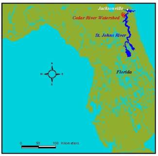
Figure 1: Cedar River Watershed
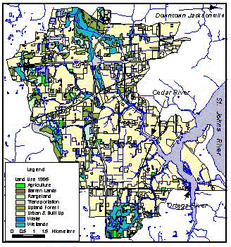
Figure 2: Cedar River Watershed Land Use Distribution
Scientists from the St. Johns River Water Management District (SJRWMD) in Florida, have identified significant concentrations of heavy metals in sediment samples taken from the Cedar River. Although some metals occur naturally in the environment, high concentrations may pose hazards to aquatic organisms. Modeling sediment and adsorbed contaminant transport within the contributing basins, can help to identify possible contaminant sources. This paper describes the first phase of a GIS-based mass balance model of overland sediment transport to the Cedar River. Parameters considered in the model include contaminant properties, elevation, rainfall, land cover, soil type, roughness, overland channel depths, flow and infiltration rates.
The Cedar River, a tributary of the St. Johns River, flows from northwest to southeast through Jacksonville, Florida. It travels approximately 5 km before converging with the north flowing Ortega River. The two rivers travel eastward another 3 km and drain into the St. Johns River. The contributing watershed, encompassing approximately 23,000 acres, is composed mainly of built-up urban areas and pine forests. Figure 1 shows the Cedar River’s contributing watershed and figure 2 shows the three rivers and land use distribution within the watershed.
SJRWMD scientists have been collecting sediment core and ponar samples at several locations within the Cedar River and at its confluence with the Ortega and St. Johns Rivers since 1995. The sampling results indicate that several heavy metal concentrations (e.g. Pb, Hg, Cu, Cd) are elevated to levels that may pose harm to aquatic organisms (Ouyang, etal. 2002). Metals are likely to adhere to soils, so runoff derived erosion provides a common pathway to water bodies.
A spatial estimation of potential soil loss for the watershed will, therefore, help to identify possible contaminant sources to the Cedar and St. Johns Rivers. The Universal Soil Loss Equation (USLE) is an empirical model used to estimate erosion, the first step of sediment transport. The objective of this project was to construct a GIS based potential soil loss spatial index model, based on the USLE equations. Once soil detachment occurs sediment is accumulated and deposited during transport within the watershed. The USLE can only estimate potential soil loss, not transport, so the index is a relative measure that will indicate where soil loss “hot spots” may exist. The index will provide useful information to aid decision makers in considering natural resource management strategies for the watershed. Soil and contaminant concentrations transported to the rivers will be considered in a second phase of the GIS modeling project.
The Universal Soil Loss Equation is an empirical model developed by Wischmeier and Smith (1978) to estimate soil erosion from fields. While the model’s limitations have been extensively documented, the equation remains the basis for a variety of soil and sediment applications including estimating watershed wide sediment transport (Renard, etal 1997). The equation is defined mathematically:
where, A is soil loss in tons per acre, R is a rainfall-erosivity index, K is a soil erodibility index, L represents slope length, S is the slope steepness factor, C is a land cover management factor, and P is a supporting practices factor. Data input, calculation of each factor and data pre-processing are discussed in greater detail below.
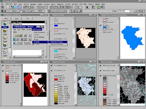
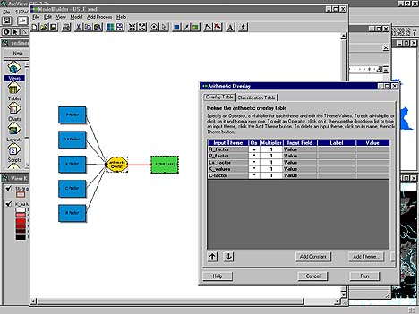
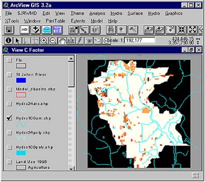
ArcView 3.2 GIS, the Spatial Analyst Extension, the Hydrologic Modeling Extension, and Model Builder were used to process input data, construct the model, and present results. Figure 3 shows the model within an ArcView project, with a single view for each equation factor’s input and pre-processed data. The Model Builder window, shown in figure 4, is the interface that allows users to build a model diagram designating the data and processes then run the model.
The USLE equation was modeled spatially by designating a raster grid for each equation factor as input parameters of the model. A mathematical overlay process multiplies the corresponding cells of each grid. Several processes can be included in one model diagram, but the Model Builder does not include the hydrologic extension processes, so pre-processing of factor grids was performed directly with the hydrologic tools, within the views.
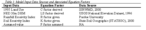
Each equation factor is used as a model input parameter. The P, K and R factors were obtained from the literature, so the only processes required were conversions to grids. C, L and S factors were derived within the model construction. Input data, their sources, and the equation factor to which they apply, are listed in table
The P factor mainly takes into account land management practices that help to reduce erosion, such as contouring on farms. Because detailed management practices were unknown, the P factor is assumed to be 1. The R factor is an index which reflects the amount and rate of runoff associated with rain and the effect of raindrop impact in terms of soil detachment (Renard, etal. 1997). An R factor was determined from the literature and set at 350 (Elementary Soil & Eng. 1995). P and R factor grids were converted from the watershed boundary polygon shapefile, containing constant cell values of 1 and 350, respectively. Constants can also be applied to Model Builder directly, but the former method was chosen for model clarity.
The K factor is a measure of soil erodibility in terms of susceptibility to detachment as well as transport, and ranges from 0.05 for low erodibility to 0.4 for high erodibility. While clays have low K values because they are not as easily detached, sandy soils also have low K values because they are difficult to transport via runoff. Silt loam soils have medium K values and soils high in silt have high K values (Ouyang and Bartholic 2001). The project area consists mainly of sandy soils and K values from 0.1 to 0.24. K factors for this grid were obtained from the STATSGO database and polygons were converted to the K factor raster grid.
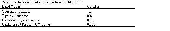
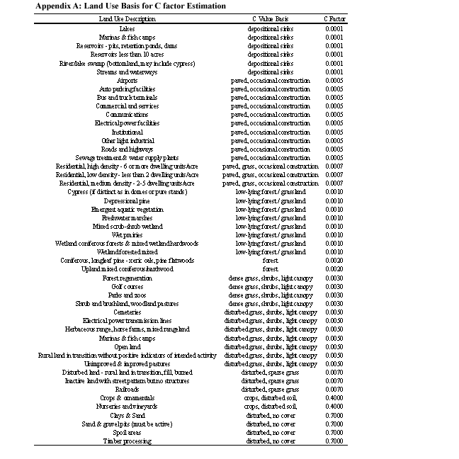
The C factor is based on crop, tillage, & timing and involves complex calculations. Since the objective is to derive a sediment source index, C values need only be relative to each other in terms of which land covers are more or less susceptible to erosion and by what degree. Estimated C values were assigned to SJRWMD1995 land use data based on values from the literature (Gardner 2001, Rehnard 1997 , Wischmeir 1978).The land use polygon shapefile was then converted to a raster grid, with a C factor assigned to each cell. Table 2 shows example C factors extracted from the literature. Appendix A lists C factor values assigned to specific land use types. Figure 8 shows the C factor distribution throughout the watershed.
The slope length and steepness factors are typically calculated together for input into the equation as:
where Lhill = slope length in meters, a = angle of slope, m = 0.5 if % S >= 4.51, 0.4 if % S is = 3.01 to 4.5, 0.3 if %S = 1 to 3, 0.2 if % S < 1, (Wischmeier and Smith 1978). The LS factor raster grid was calculated using the following processes, all based upon the Digital Elevation Model (DEM) as initial input data.
1. ArcView Spatial Analyst Processes to derive slope angle, S Factor:
a. derive slope angle in degrees from DEM
b. convert slope angle from degrees to radians, required input for map calculator trig functions (S factor grid)
c. derive slope angle percentages to calculate m values
2. ArcView Hydrologic Modeling Extension Processes to derive slope length, L factor grid:
a. fill DEM sinks
b. calculate flow direction grid
c. calculate uphill flow length grid (L factor grid)
d. create new analysis mask from map query which includes only flow lengths greater than 122 meters(1)
3. ArcView Spatial Analyst Process to calculate LS Factor:
a. enter LS factor grids and LS equation into map calculator to calculate LS factor, using equation 2:
([Flow Length Grid] / 22.1).Pow( [M Value Grid] )* [Slope Radians Grid].Sin.Pow( 2 ) * 65.41+ [Slope Radians Grid].Sin * 4.56 + 0.065
4. ArcView Spatial Analyst Model Builder process to calculate A.
a. Designate input model data: add each factor grid
b. Designate model process as arithmatic overlay: multiply all grids
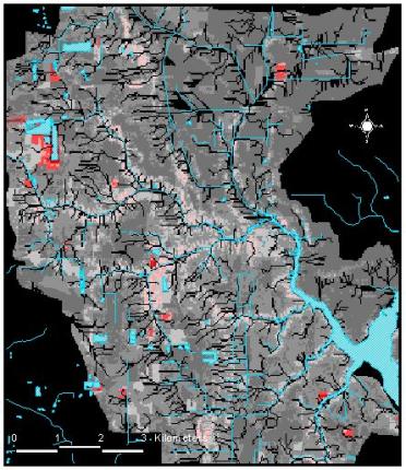
Once the equation factor grids were created and designated as model input parameters, the model was run and the resulting grid was log transformed and reclassified for comparison of values and presentation of results. The reclassified values will serve as an index to be used as an initial indicator of potential sediment source “hot spots”. As such, preliminary results show that potential soil loss is typically greatest along the steeper sloped banks of tributaries. Other “hot spots” are dispursed throughout the basin and are typically associated with high erosion potential land uses, such as spoil areas. Further investigation of model parameter values and acquisition of empirical data are needed before the model can be calibrated or verified. Given that the watershed landscape consists mainly of gradual slopes and built up urban land cover, these preliminary results indicate that the model is simulating real world processes, (eg. low erosion rates on paved and gradual sloping surface). Figure 6 shows the final soil loss potential index grid overlayed with hydrography. Referring back to the land use map, (figure 2), it is easy to match the red “hot spots” with erosion sensitive land use types.
Now that the model has been constructed within ArcView 3.2, parameter inputs can be updated and/or completely replaced without the need to access programming code as with ArcInfo and non-GIS based models. This makes the model user friendly for all GIS Analysts and those scientists, engineers and planners with some GIS background. The model can also be customized with pop-up windows to simplify use even further for those with no GIS background. When Model Builder is available in ArcGIS, it may be worth converting the model to ArcGIS 8.1 to allow access to SDE data. Having access to more functions in Model Builder, such as the Hydrologic Modeling Tools, would allow more of the model to be automated and increase user friendliness.
The objective of this project was to use ArcView 3.2 and the Model Builder to construct a simple model to spatially estimate potential soil loss areas within the Cedar River Watershed. Model results are consistent with observed erosional processes suggesting that further development of the model would yield a useful planning tool.
1. Research indicates that slope length typically does not exceed 122 meters (400 feet) before runoff accumulates into a defined channel (Renard 1997). The USLE does not apply to channels, so excessive flow lengths were excluded from analysis by creating a new mask grid from the flow length grid (using map query) where values were less than 122 meters. This grid was used as the L factor grid to calculate LS.
John Higman, Ying Ouyang, Dean Campbell, Awes Karama, Getachew Belaineh, Tim Cera, Mark Atkins, Troy Keller, Paul Finer, and Dean Dobberfuhl are greatfuly acknowledged for their scientific and technical support.
Elementary Soil & Engineering 1995, Purdue University Web Site, Rainfall Erosivity Index http://danpatch.ecn.purdue.edu/~wepphtml/wepp/wepptut/jhtml/imagedir/usa.gif
Gardner, D. 2001. Lecture 23: Soil Erosion, Web Site, Texas A&M University – Kingsville
Ouyang, D. and Bartholic, J. 2001. Web-Based GIS Application for Soil Erosion Prediction, Proceedings of An International Symposium – Soil Erosion for the 21st Century, Honolulu
Ouyang, Y,. Higman, J., Thompson, J., O’Toole, T., and Campbell, D. 2002 Characterization and spatial distribution of heavy metals in sediment from Cedar and Ortega rivers subbasin. Journal of Contaminant Hydrology 54. Elsevier
Renard, K.G., Foster, G.R., Weesies, G.A., McCool, D.K. and Yoder, D.C. 1997. Predicting Soil Erosion by Water:A Guide to Conservation Planning With the Revised Universal Soil Loss Equation (RUSLE). U.S. Department of Agriculture Handbook No. 703
Wischmeir, W.H. and Smith, D.D. 1978. Predicting rainfall erosion losses: a guide to conservation planning. Agriculture Handbook 537. USDA-ARS