
|
|
Geospatial Applications Laboratory
Center of Higher Learning
University of Southern Mississippi
An Approach to Large Area
Pin-Map Problems
Bart Pittari, Paul Crocker
Jim Matthews, Mitch Tinsley
Geospatial Applications Laboratory
Center of Higher Learning
University of Southern Mississippi
This paper describes the rule development process and software issues encountered in the development of a geospatial expert system for a large (1.25 x 10⁵ km2) area. The analysis included expert interviews and a neural network classification to develop rule hypotheses. The hypotheses were then statistically tested against random occurrence. Hypotheses testing significantly above or below random occurrence were used to produce GIS coverages that were combined using a weighted union to produce a coverage representing areas likely to exhibit the phenomena being modeled. This technique is felt to be applicable to a wide variety of pin-map problems.
Law enforcement agencies have long used pin maps to perform spatial analysis. Different color pins were used to denote different crimes or incidents, and their grouping used to identify hot spots of activity. The advent of digital data and its processing has not only led to the automation of this type of spatial analysis, but the combination of this type of data with Geographic Information Systems (GIS) has led to the ability to identify additional areas with similar characteristics that have a high potential for crime.
The geospatial expert system approach described in this document is applicable to all pin-map type of data. Since this paper deals with Law Enforcement Agency Sensitive data, no direct reference is made to the actual nature of data that was involved in this process.
The first step was to interview experienced law enforcement officers regarding the activities being modeled in this exercise. A questionnaire was developed based upon preliminary interviews with selected personnel. This was then distributed to a wide variety of law enforcement personnel with experience in the activity being modeled. From these interviews, policy/procedural information was developed on how and what they look for, etc. The questionnaire was followed by in-depth interviews with personnel having a minimum of five years experience. The information from the questionnaires and interviews were summarized and a profile was developed to identify potential relationships.
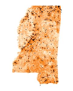
Existing state wide pin-map data was obtained and processed and all available state-wide GIS data was collected. Existing data consisted of a variety of layers including transportation (roads, railroads), hydrology (perennial streams, intermittent streams, water bodies), and land use (soil data, land type). Most of the state data was taken or derived from the Mississippi Automated Resource Information System ( MARIS ), which serves as a data clearinghouse for the state of Mississippi. Soil data was obtained from the Soil Survey Geographic Database ( SSURGO ) and from State Soil Geographic Database ( STATSGO ).
Existing pin map data consisted of 365 points covering a 5-year period of time that represented criminal activity, plus an additional years worth of data (81 points) that was collected after our study began and used in a blind test to evaluate our prediction system. The processed data were input to a neural net along with random points to identify potential rules by looking for relationships between the pin-map and GIS data that differed from random chance. Neural net results were then used to develop threshold levels for what's considered random. In order to ensure randomness, 10 sets of random data points were generated within the state boundary and used to test for patterns by comparing the ratio of the historical point data vs. random points.
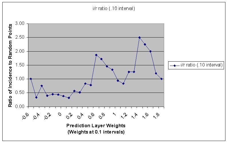
Figure 1a - I/R Ratio plot of incidence and random sites. Random is considered where the line crosses the Y-axis at 1.00 - anything greater than that value + 10% is considered likely area and anything less than that value - 10% is considered unlikely area
A weighted union of the rules was used to produce the decision layer. This was accomplished by executing an Arc Macro Language (AML) script that performed a weighted union of 16 coverages. A 17th coverage with a weight function of 0.0 was added to the union. This was a state of Mississippi boundary polygon added to fill holes in the event that there were areas with no polygonal coverage in the final outcome, and to trim buffer zones that extended into neighboring states or the Gulf of Mexico. The union performed additions (cov1 + cov2 = out1; out1 + cov3 = out2 ...). The higher the weight number in the final coverage, the more likely the phenomenon is to occur in that area. Table 1 provides an example of rules and selected parameters.
|
Parameter
|
Buffer/Class
|
I/R
|
Area of State (%A)
|
Weight
|
|
Streams
|
500 m
|
0.50
|
50.5
|
-0.55
|
|
Roads
|
300 m
|
1.50
|
45.8
|
+1.30
|
|
Land Use
|
Agriculture
|
0.25
|
20.5
|
+1.56
|
|
Road Density*
|
2.5-6.5 km-1
|
1.25
|
33.0
|
+1.20
|
|
Clustering**
|
7500 m
|
5.07
|
25.0
|
+1.40
|
A dissolve function was then performed on the coverage produced by the union to simplify the coverage. The resultant coverage was highly fragmented and contained just over three million polygons, ranging in size from 0.0005 km2 to 62.3 km2 The mean and standard deviation of the polygonal areas were 0.04 km2 and 0.14 m2 respectively. The largest polygons were water reservoirs. The maximum possible weights were -0.66 and +2.49, while the actual range was -0.16 to +2.45.
The final step in producing the prediction layer in vector space was to relate the polygon weights resulting from the union of the rules to the likelihood of finding the pin-map data of interest. The weights were based upon a incidence-to-random ratio and do not represent probabilities. This was done by taking the historical data and an equal set of generated random points and performing a spatial join to the prediction layer with each of them. The weight of the polygons that both sets of points fell on were then ranked and graphed on a quantile plot. The range was determined by the separation of values as is shown below in Figure 1b.
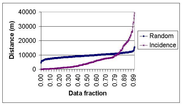
Figure 1b - An example of a quantile plot where the random points and historical data points were spatially overlaid on a coverage (in this case road density) to determine non-random values.
The number of sites and random points diminish as the upper and lower weight values are approached. This results from the fact that polygons with extremely low or high weights, those representing the tails of a histogram, comprise less area than those in the mid-range. Therefore, fewer points are inherently to be found in the areas of the map with values representing the tails. This translates into a very small sample size from which to calculate ratios.
As would be expected, a very high computational price is paid for the topology of vector computation. Vector coverages ballooned to a total of 60 GB in size and took appriximately 2 weeks for processing. The vector coverages used as input were up to 1.5 GB in size, the intermediate union coverages totaled 40 GB, and the final union before a dissolve was performed was a 10 GB file. The total hard drive space required just to store the files is approximately 60 GB, and several times that amount is required to perform the computation. Run times for a single buffer on a single coverage ranged from under an hour to over a day in duration.
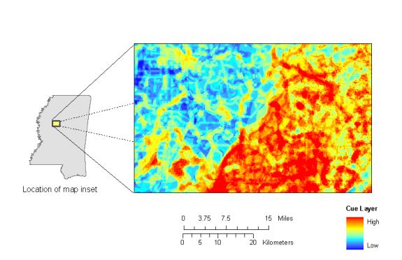
The sixteen vector coverages representing the rules were rasterized to a 50-meter grid and the same weighted union performed using the GRID function of Arc Workstation. The union took approximately 2 hours of computer time to complete and resulted in a 300 MB file. The resulting raster solution, as is illustrated above in Figure 2, was just as detailed as it's vector-produced counterpart.
In view of these difficulties it is clear that computations of this magnitude should always be performed with raster formatted data, unless there is a specific need for the attributes associated with vector data. In the present investigation, the topology of vector computation were of little value in interpreting the final results and were not warranted.
Geospatial expert systems based upon multiple weak rules can have significant predictive ability. For example, this investigation identified areas in Mississippi that were four times more likely than random chance of the modeled parameter occurring. This is considered to be our most significant finding. This, together with using the neural net, comprise a process that is used to develop the expert system rule set which is felt to be directly applicable to virtually any type of pin-map data.
There is often a negative connotation associated with the use of neural networks, because the intermediate steps in their solution process cannot be ascertained. However, the current investigation found a neural network to be an extremely valuable analysis tool. Since most investigations are limited by the availability of data, all available, relevant GIS data was input to a neural network and a classification analysis performed. The results, in combination with the information obtained by interviewing experienced law officers, were used to formulate a set of rule hypotheses. The rule hypotheses were then individually tested against random chance, and sixteen of them were identified as statistically significant predictors. These surviving hypotheses were assigned weights on the basis of their performance against random chance and combined in a GIS by a weighted union to produce a map (solution coverage) predicting areas in the state that were likely to exhibit the phenomena modeled. The predictive ability of the solution coverage was then compared in a blind test against data after its development. The statistically verified rules, when combined by a weighted union, outperformed both a neural network prediction and the traditional approach, which consists of going to where they found it before and using pure instinct, used by law enforcement.
The topology associated with vector format coverages made the statistical development of the rule set and solution coverage production by the weighted union extremely labor and computer intensive. In contrast, computation in raster format was computationally economical. The neural network classification analysis was also computationally economical. These factors, and the superior predictive ability of the statistically developed rules, suggest the following steps for the development of a solution coverage from pin map data.
- Interviews to determine perceived rules
- Acquisition of all available GIS coverages for the study area
- Acquisition of historical pin map data
- Neural network classification of coverages as predictors to pair down data to relevant rules
- Combine interview results and neural network classification to develop rule hypotheses
- Statistically evaluate rule hypothesis by comparison to random chance (raster format)
- Weighted union of rules (raster format)
- Evaluation of the solution coverage against data not used in rule development