The Reservoir Sedimentation Survey Information System (RESIS) is the most comprehensive database of reservoir sedimentation rates in the world, comprising nearly 6,000 surveys for 1,819 reservoirs across the United States. The use of this database has been limited by the lack of precise coordinates for the reservoirs. Many of the reservoirs postdate current USGS topographic maps and have only township and range coordinates. This paper presents a method scripted in Esri's ARC Macro Language (AML) to locate the reservoirs on 30-meter digital elevation models using available reservoir information. The script then delineates the contributing watersheds and compiles several hydrologically important parameters for each reservoir.
Many studies have compared the characteristics of watersheds to the rates of sediment production from those watersheds (Neil and Mazari, 1993; Verstraeten and Poesen, 2001; Farnham, et al, 1966; Flaxman, 1966). Sediment output is usually measured as suspended load at established gauging stations or by estimating the accumulation rate of sediments in man-made reservoirs through repeated surveys of bottom bathymetry. An integral part of such investigations is the characterization of the watershed above the sampling point. This almost always involves a collection of parameters describing watershed topography and often includes descriptions of watershed soils and land cover as well. Most previous research has used intensive fieldwork or tedious map and aerial photo interpretation to measure these watershed parameters (Paulet, 1971). Because of the extensive labor involved in such investigations, the number of individual sites considered is limited and rarely has exceeded 30 sites per study. With modern datasets derived from digitized maps and remote sensing instruments describing topography, climate, soils, and land cover for the continental United States (US), many of these parameters can be measured using a geographic information system (GIS). Especially when sediment output from a large number of basins is already known, GIS can aid in the characterization of the watersheds and permits much larger-scale studies than were previously possible.
This paper outlines the method used to "geolocate" and characterize the hydrologic properties of 537 watersheds located above man-made reservoirs catalogued in the Reservoir Sedimentation Survey Information System (RESIS). Using Arc/Info 8.0.2 and the Arc Macro Language (AML), this automated procedure uses available information about the watersheds to locate the point on a 30-meter digital elevation model (DEM) that has area and elevation characteristics most similar to those recorded in the database. Once the best location for the dam is determined, the watershed boundaries are derived and used to clip freely available GIS grids that describe the topography, soils, climate, and land cover of those watersheds.
Starting in the 1940's, several programs were developed that ultimately caused a boom in reservoir construction in the US. The Flood Control Act of 1944, the Pilot Watershed Program, begun in 1953, and Public Law 566, enacted in 1954, led to the construction of several thousand floodwater retarding and multi-purpose structures across the US. These programs were immensely popular and have led to a significant change in the hydrologic and sedimentologic cycle for the United States (Roehl, 1966).
The most common uses of reservoir capacity in this country are for flood control, drinking water supply, recreation, and hydroelectric power generation. All of these uses can be severely limited as reservoirs fill with sediment. In response to the growing concern about reservoir siltation, the Subcommittee on Sedimentation Interagency Advisory Committee on Water Data began compiling sedimentation surveys for over 1,800 reservoirs across the United States. The result of this compilation is RESIS, the most comprehensive database of reservoir sedimentation in the world. The database contains nearly 6,000 surveys for 1,819 reservoirs across the contiguous United States (excluding Florida and Maine).
Periodically, the US Department of Agriculture (USDA) summarizes the known reservoir sedimentation survey data. The sediment data in RESIS for the period ending in 1965 were interpreted by Dendy et al. (1973). This summary included approximately 3,500 surveys. For their compilation they divided the US into 79 sub-basins and summarized the results for each sub-basin. The data were summarized again for the period ending in 1975 by Renwick (1996). This summary included an additional 1,500 surveys. Renwick (1996) used nearest town locations recorded in RESIS to approximate reservoir locations to within 20 to 50 km. Local relief in the vicinity of the reservoir was determined by calculating the average value of local relief within a 5 km radius of the town nearest the reservoir using topographic information taken from 3-second DEMs. There is no published comprehensive analysis of the nearly 500 surveys entered into the database since 1975.
The database has recently been incorporated into a new database management package (Corel Paradox v9.0), given a new interface, converted to metric units, and the geographic coordinate information for most of the reservoirs has been updated. At the beginning of 1999, the database had latitude and longitude information for less than 800 of the 1,800 reservoirs in the database. Less than 350 had been "geolocated" on DEMs (enabling the delineation of the watershed). This made any large-scale use of RESIS with GIS systems impossible.
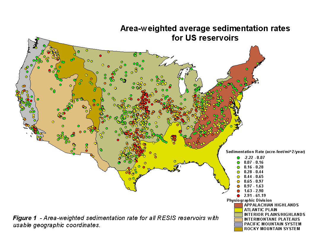
With the ever-increasing number of sub-kilometer resolution databases of recent years, there is a growing need to find more accurate positions for these reservoirs. Recent work has increased the number of reservoirs with reliable coordinates to 1,296. A map of the area-weighted sedimentation rates (acre-feet mi-2 yr-1) for all of the reservoirs with usable geographic coordinates is shown in Figure 1.
Five large-scale datasets were used in this study; each is described below. They provide excellent resources for large-scale sedimentologic and biogeochemical studies within the United States. The first and most integral dataset used was RESIS, described in the previous section.
The second was the State Soil Geographic Database (STATSGO) for the contiguous United States (USDA, 1994). Developed by the USDA, STATSGO summarizes local soil surveys on a national scale and provides many attributes, including organic matter content, K-factor (soil erodibility as defined in the Revised Universal Soil Loss Equation (RUSLE)), grain size information, available water capacity, and permeability. A version of STATSGO that had been summarized on 1 km grid resolution and is currently available at the address: http://water.usgs.gov/lookup/getspatial?muid was used to compile soil erodibility and organic matter content values. This version of STATSGO was convenient because it included the information necessary for this study, but other versions of STATSGO are available through the USGS and USDA websites.
The third relevant database was the PRISM (Parameter-elevation Regressions on Independent Slopes Model) rainfall database (Daly et al. 1994), maintained by the Oregon State Climate Center. The downloadable maps from the PRISM website at http://www.ocs.orst.edu/prism/prism_products.html show mean annual rainfall for the United States. PRISM is a regression model that interpolates rainfall in mountainous regions where orographic effects determine rainfall patterns.
The fourth database used in this study was the USGS National Land Cover Dataset (NLCD) (Vogelmann, et al, 2001). This dataset was generated through analysis of 1992 Landsat thematic mapper imagery and consists of 21 classes of land cover at a resolution of 30 m. Currently, these data are available online from the USGS at http://landcover.usgs.gov/natllandcover.html.
The fifth dataset used was the National Inventory of Dams (NID). The NID contains general information, including reservoir capacity, dam height, construction date, and geographic coordinates for every dam in the United States that is over 6 meters tall. This database was previously available online at the following address: http://crunch.tec.army.mil/nid/webpages/nid.cfm. However, national security concerns have led to its removal from public access indefinitely. This database was used in two ways. First, it was used during the preprocessing of the RESIS database to supplement the geographic coordinates of the reservoirs that were described in both databases. Second, the NID was used to determine the extent of reservoir "nesting" by recording the number of reservoirs present within the watershed area of each reservoir.
Fewer than 900 reservoirs in the RESIS database had geographic coordinates that could be used without alteration for input into the geolocation program. A small number (334) had previously been manually located on topographic maps and given new coordinates that would match their location to their watershed "outlets" on standard USGS DEMs. For the remainder, several techniques were applied to determine "starting coordinates" that could be used in the geolocation program detailed below. The methods are presented in the order they were applied. The method that was considered most accurate was used first, and subsequent methods were only used for reservoirs for which the prior methods could not provide coordinates.
The first method involved matching reservoirs in RESIS to those in the NID based on reservoir name, and the recorded city, county, and state in which the reservoir is located. It was assumed that the coordinates in the NID are more reliable than those in the RESIS database and visual inspection of coordinates of a subset of dams confirmed this. 735 reservoirs were assigned improved coordinates in this manner, replacing many of the less precise coordinates recorded in RESIS.
If latitude and longitude were not provided in either the NID or RESIS databases, the second method involved using the recorded Public Land Survey (PLS) coordinates (if available) to determine approximate latitude and longitude. This was performed using a program called TRS2LL developed by Marty Wefald, that returns the latitude and longitude for the center of a PLS section for the majority of the US. The program is available at http://www.geocities.com/jeremiahobrien/trs2ll.html. Because latitude and longitude are for the center of the section in which the reservoir was located, these coordinates may be in error by as much as 0.7 miles. There are 50 reservoirs that were assigned new coordinates with this method.
The third method of "starting coordinate" determination was used when the first two methods were not usable. This method uses the "nearest post office" value in RESIS. Like the method used by Renwick (1996), the "places" database of the USGS was queried for the coordinates of the town center for the nearest post office. These coordinates were assigned as the reservoir's "starting location." The previous methods were not always applicable and the nearest post office is known for nearly every RESIS reservoir. This method represents the worst-case scenario for starting coordinate determination. The estimated positional error of this method is variable, depending upon which part of the country the reservoir is in; the error is higher in the western states because the relative density of post offices is lower than in the eastern US. This method of starting point determination was required for 427 of the reservoirs in the RESIS database.
The original plan for implementing this GIS was to locate the reservoirs by hand and digitize the coordinates at the top center of the dam. It soon became apparent that this would not be as easy as anticipated. Many of the reservoirs in the RESIS database do not show up on standard 7.5-minute topographic quadrangle maps. This was due to at least one of three main reasons: 1) the most up to date map available had not been revised since the construction of the reservoir, 2) the reservoir was too small, or was dry for too much of the year to show up on the aerial photos used to construct the original maps, or 3) the reservoir had been drained or completely filled with sediment at the time of the construction of the topographic map. Thus, an alternative method was needed for the geolocation of these reservoirs if they were to be characterized in a GIS.
The following section describes the methods used for geolocation. The hypothesis behind this method is that, for the purpose of geospatial data gathering when geolocation by hand is impractical or impossible, collecting data from a "similar" watershed within close proximity of the dam provides in most cases a reasonable description of the watershed above the dam. A "similar" watershed is defined as a watershed that lies at the same elevation and has the same total area as the watershed described in the RESIS database. Without rigorous hand checking of the data sets, this "similar" watershed is indistinguishable from, and may be the same as, the actual watershed of the dam. The following sections will describe this method and present the results of an examination of the variability of several GIS-derived parameters between nearby watersheds of similar size and at similar elevations.
To delineate the watersheds, it was necessary to have a representation of the local topography. In this case, a DEM, which represents elevation as a continuous grid of elevation values, was chosen, as they are the most widely available forms of topographic data for the US and are easily used for topographic characterization. The USGS has digitized most of the 7.5-minute topographic maps for the continental U.S. These have been made freely available on the internet as DEMs. Though a large-scale seamless DEM for the continental US (The National Elevation Dataset (NED)) was made available during the course of this research, the funds for its purchase were not available. The necessary 7.5-minute grids were acquired from the USGS WebGLIS (Global Land Information System) site developed at the Earth Resources Observation Systems (EROS) Data Center and later from www.gisdatadepot.com when the responsibility of DEM distribution was transferred from the USGS to a private company. The DEMs were stored and most GIS calculations were performed on a SUN mainframe computer. Esri's software packages Arc/Info 8.0.2 and ArcView 3.2 for UNIX were installed on a 400MHz SUN Enterprise 6500 running SunOS version 5.8.
The AML script was originally designed to run on only small watersheds - those with a watershed area of approximately 250 sq. km or less. Most natural watersheds of this size are likely to be contained on a 3x3 mosaic of 7.5-minute, 30-meter resolution DEMs (at least in the continental US). To construct these 22.5-minute DEMS, a polygon coverage showing the name and location of all USGS 7.5-minute topographic maps was acquired. This coverage contains the USGS Quad-ID code, which is based on a grid numbering scheme that can be reproduced with a fairly simple algorithm. This permits the creation of an AML script that returns the name of the 8 quads surrounding a given 7.5-minute quad. A modified version of this script was used to create a mosaic of the area grids around the best available starting coordinates for the dam.
Once the DEMs were properly mosaicked, the next step was to "fill" them, eliminating small errors in the DEM called "sinks", which consist of a cell or small group of cells lower than all surrounding cells. Generally, these sinks do not represent the true topography (and thus hydraulic flow) of the area, though karst terrain and glacial till plains are examples of areas where these may occur due to true topographic expressions (few reservoirs were located in such places, so no effort was made to insure the preservation of true sink holes or kettles).
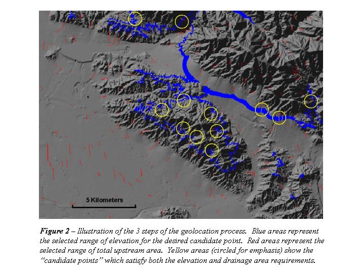
Once the area DEM was prepared, a "spillpoint" was determined for each reservoir. The information provided in RESIS for each reservoir made this possible. Knowing the approximate location of the reservoir, the minimum and maximum elevation in the watershed, the elevation of the dam spillway, and the watershed area allows fairly accurate location of the spillpoint on a topographic map or DEM by hand. With the techniques in the following paragraphs, this procedure was automated.
One problem with identifying the true edge of the dam was that on some DEMs the reservoir appeared as a topographic feature (i.e. a large flat area at the elevation of the spillway), while other DEMs instead showed the original topography underlying the reservoir surface. Thus, there was no consistent automatic way to identify which point along the stream course was the true spillway. So, the program looks first to see if the lowest elevation in the watershed is recorded (it is not for all reservoirs in RESIS) and if it is not it uses the spillway elevation. In some cases this meant that the watershed was delineated slightly above or slightly below the true spillway. But, the mean watershed values for parameters like slope, soil properties, and land-cover are not significantly affected by these deviations. Using this elevation, the DEM is queried for elevations falling within �10% of this value. This produces a binary grid with "rings" of potential reservoir sites around high and low features (the areas marked in blue in Figure 2).
With the majority of the DEM area eliminated as potential dam locations, the next task was to further limit the search using total watershed area. Thus, the Flowdirection and Flowaccumulation commands were run on the area DEM of each reservoir to define the watershed area for every point on the DEM. Then, using the total watershed area recorded in RESIS, this grid was queried for accumulation areas within 10% of this value, producing "strings" along stream courses showing potential gridcells for the dam location (the areas shown in red in Figure 2).
Finally, these two binary grids were multiplied to produce a final binary grid. The points on this grid represent "candidate points" with an elevation and contributing area within 10% of the true values for the watershed. Because of the 10% window of elevation and watershed values selected, many of the candidate "points" were actually composed of strings of gridcells. These are shown as the small strings of yellow gridcells (circled for emphasis) where the red and blue areas overlap in Figure 2. The final "spillpoint", defining the best guess for the location of the dam, was chosen as the candidate point closest to original starting coordinates. In some cases, this meant that a point with an elevation and/or contributing area having an error of 10% was chosen despite the fact that a more suitable point (i.e. a point with a lower deviation from the recorded value) may have existed just a little further from the starting point. Modifications were made to a subsequent version of the AML script to alleviate this problem. Additionally, the tolerance level for both elevation and contributing area (currently 10%) can be modified in the current version of the algorithm based in part on estimated terrain complexity, which is discussed more in a later section, to adaptively reduce the number of candidate points.
Once the spill point was defined, the Watershed command was used to delineate the watershed with the DEM. This command creates a binary grid that can be converted to a polygon coverage. This polygon was used to clip the DEM of the local area so that parameters could be collected describing the watershed topography (e.g. mean slope, hypsometric integral, relief, minimum and maximum elevation, maximum flowpath length, and watershed area). For most watersheds, it was observed that the 30-meter resolution of the DEM was sufficient for characterization of the general topography of the watershed. However, for watersheds with areas less than ~0.5 sq. km (n = 52 for this study), the derived topographic parameters may not be reliably represented at this resolution.
The watershed polygon was also used to clip several additional grids (described above) characterizing soil, rainfall, and land cover. These values were added to a new database file keyed to the original identification numbers in the RESIS database.
In some cases, the DEMs were provided in inconsistent vertical units (i.e. sometimes in meters, sometimes in feet). It was necessary then to convert the 9 grids to be mosaiced into one consistent set of units. Because the RESIS database was compiled in English units and the majority of the DEMs used feet for elevation units, all metric elevation grids were converted to English units. Watershed values such as relief were later converted to meters.
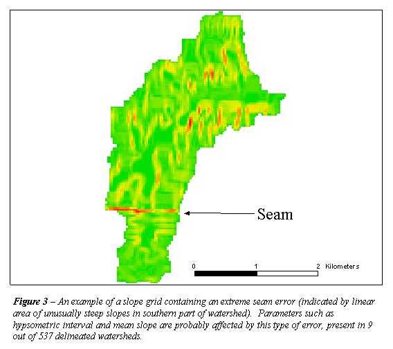
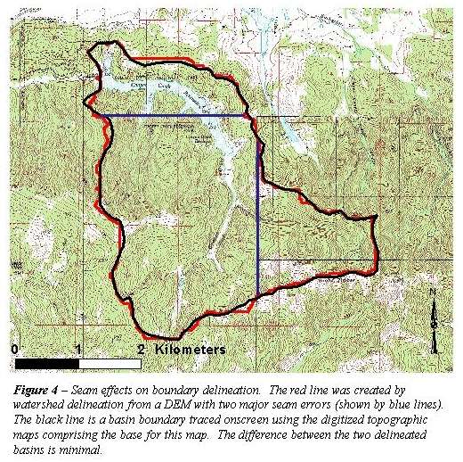
In addition to dealing with inconsistent vertical units, another well-known problem was encountered: DEMs often do not patch together seamlessly. Figure 3 shows an example of a slope grid generated from a watershed DEM containing one type of seam error. In this case, the DEM to the south shows elevations along the valley bottom near the seam to range from 1161 to 1165 feet above mean sea level (msl). The DEM to the north shows elevations in the valley bottom near the seam to range from 1135 to 1141 feet above msl, creating an artificial 20 to 30 foot "cliff" in the watershed. This type of seam error occurred with varying severity in 44 cases. However, we found that the watershed boundary was in no case significantly affected by the presence of this seam. Figure 4 shows an example. The topographic map for this watershed is overlain by two boundaries. The geolocation program derived the red boundary while the black boundary was traced on screen over a scanned topographic map in ArcView. The two blue lines indicate the locations of two level 3 seams. There is no visible effect on the boundary of the watershed in the vicinity of these seams.
In many cases, another type of seam error occurred where adjacent DEMs did not meet exactly, leaving a gradually widening gap along the seam between them. This was fixed with an edge-matching algorithm that calculates a moving average using a 4x4 window for any blank cells between the adjacent DEMs. This leads to some minor topographic aberrations, but they are assumed to have a negligible effect on the mean watershed values for the topographic parameters examined.
Another phenomena encountered while compiling the watershed DEMs was a "granularity" or a mesh of abnormally high and/or low values imposed upon the natural topography. This effect is due to the sparse sampling grid that was used for the construction of some DEMs, and is particularly noticeable in places like Ohio that have gentle, repeating topography (though it has been seen in much more topographically complex areas like Boulder, CO). While in extreme cases this may lead to a slight increase in the mean slope of the affected watershed the effect was generally assumed to be insignificant.
There were 1,490 reservoirs with appropriate information for geolocation, though only 580 watersheds were ultimately delineated and characterized. 384 reservoirs could not be located because no candidate point satisfied the requirements of the geolocation program. In most cases, this was due to incorrect information (such as minimum watershed elevation) recorded in the RESIS database. The remaining watersheds were not delineated because one or more DEMs for the area surrounding the starting coordinates recorded for the reservoir had not been acquired at the time of program execution. While every effort was made to collect as complete a set of DEMs as possible, DEMs for some areas were still not available at the WebGLIS ftp site at the time the data were acquired.
While many of the watersheds have had their positions verified on topographic maps it was impossible to verify the positions of many of the smaller reservoirs. This section outlines an experiment to determine the extent and type of potential errors encountered by delineating a watershed that lies close to, but is not, the watershed for a particular reservoir.
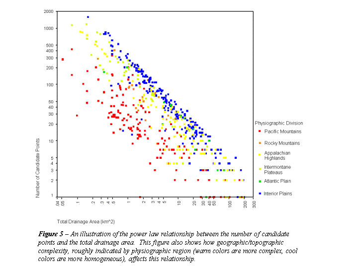
Figure 5 shows the number of candidate points (as determined by the geolocation script) plotted versus the recorded drainage area in RESIS. It shows that a strong negative logarithmic relationship exists between these values. Given a relatively constant nine-quad (22.5-minute) area, the maximum number of watersheds of a given size is constrained. As the size of the watershed in question increases, the number of potential watershed candidate points in the nine-quad grid is reduced.
The scatter away from the trend in Figure 5 is not random but is geographically controlled. Almost all of the points that fall distant from this trend are located in the Pacific Mountains. In fact, the reservoirs in mountainous areas fall consistently further from the trend line than do reservoirs in flat regions. An examination of several DEMs for the areas surrounding reservoirs close to and far from the line shows that the number of candidate points per unit drainage area seems to be controlled predominantly by "terrain complexity" (though it is also controlled to a lesser extent by the relationship of the minimum watershed elevation to the mean elevation in the chosen DEM area). In other words, an area with steep mountains bounded by broad flat plains or an area with rolling hills cut by a large floodplain will typically have a smaller number of watersheds that satisfy both the elevation and watershed area constraints imposed by the geolocation program. Though more complex terrain areas have fewer candidate points, reducing the chances of picking the wrong watershed, the consequences of choosing the wrong watershed in topographically complex areas can be significantly greater than in more homogenous regions.
To quantify this effect, three areas were chosen to represent terrains considered simple, moderately complex, and complex. The level of complexity was assumed to be represented by the distance each point fell from the observed power law relationship shown in Figure 5. This distance has since been quantified by fitting a line through the upper limits of the data scatter with approximately the same slope defined by this upper bound. The "complexity" number was then calculated as the difference between the value predicted by this line and the true number of candidate points divided by true number of candidate points (Equation 1).
C = (Ca - Cp) / Ca, where Cp = 25670A-0.9017 (1)
For each area, the ten (10) candidate watersheds (as defined by the "candidates" coverage produced by the geolocation program) falling closest to the best available coordinates for the actual reservoir were chosen. Once delineated, each watershed was characterized by a set of relevant parameters chosen to illustrate the potential for misrepresentation of the watershed.
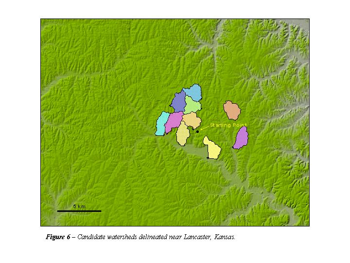
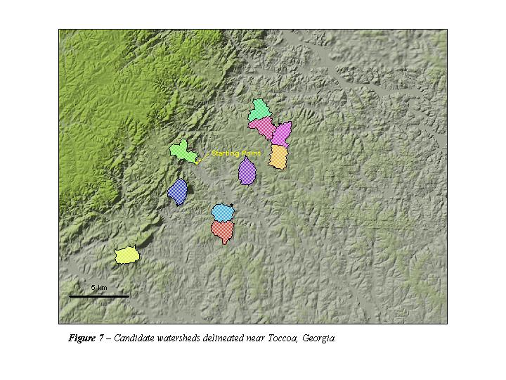
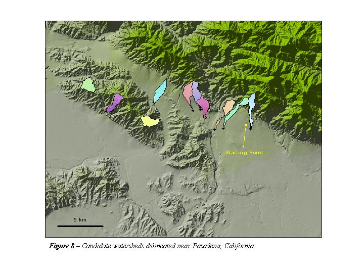
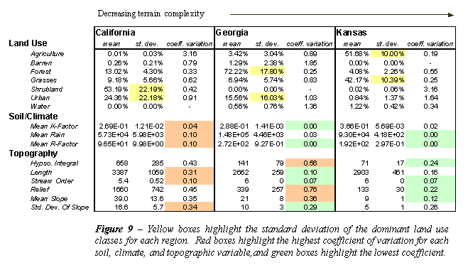
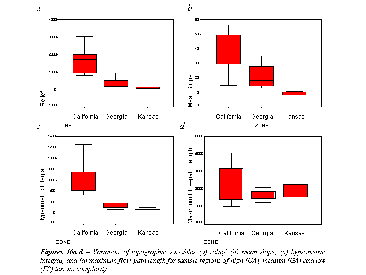
The three area DEMs chosen were centered on the Lancaster, Kansas quadrangle, the Toccoa, Georgia quadrangle, and the Pasadena, California quadrangle. The locations of these three areas on the complexity plot (Figure 5) are indicated. The three areas represent complexity values of 0.37, 3.4, and 15.8 for Kansas, Georgia, and California, respectively. The locations and boundaries of the 30 watersheds considered are shown in Figures 6, 7, and 8.
The average distance of the nearest 10 candidate watersheds to the starting coordinates increases with terrain complexity. Near Pasadena, the watersheds are spread out along the foothills of the ranges and the distance from the starting point to the furthest watershed exceeds 18 km. The watersheds near Lancaster, however, are clustered tightly around the starting point and the distance between the starting coordinates and the most distant of the 10 nearest spillpoints is approximately 4.6 km.
Some summary statistics for each region considered in its entirety as well as the statistics describing the 10 watersheds from each area are presented in Figure 9. The variability of nearly every topographic and climatic parameter characterized for the watersheds near Pasadena, California is higher than that seen for the watersheds near Lancaster, KS. The mean values and level variation for the Toccoa, Georgia area fall pretty consistently between those for the other two
Figures 10a-d show boxplots for four of the topographic parameters considered. All four plots illustrate the more dramatic topography seen in the California watersheds compared to the Kansas watersheds. Though the standard deviation for the California watersheds is large, the values for relief, mean slope, and hypsometric integral for all California watersheds is distinguishable from the 10 Kansas watersheds. The Georgia watersheds are more or less in between those of the other two regions for all of the parameters shown, though the variation of total stream length (L) for the watersheds of each region shows some overlap, suggesting that basin length is not as subject to the effects of terrain complexity as are some of the other parameters.
Examining the land cover values, we see that the coefficient of variation (standard deviation divided by mean) for the dominant land classes in each area is a function of that area's complexity. Shrubland is the dominant land cover in the mountainous watersheds of the Coastal Ranges of Southern California and shows a standard deviation of ~22%. The dominant land cover of Georgia, forest, shows a standard deviation of ~18%. Dominant land cover in the Kansas watersheds was divided between agriculture and grasses (pasture). The standard deviation for each is about 10%. The sum of the standard deviations and coefficients of variation for all land cover classes of each region is also shown. This presents a measure of overall variation of land cover in each region. This also illustrates the observed pattern of greater variation in the California watersheds and lesser variation in the Kansas watersheds.
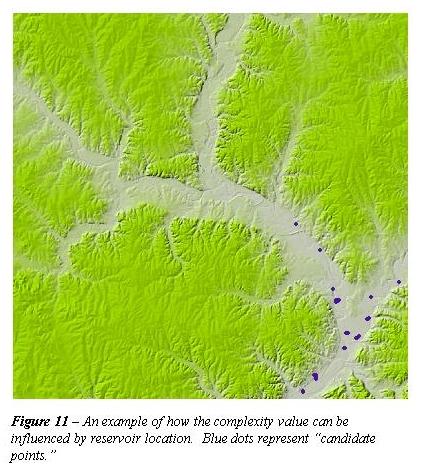
This complexity factor is merely an approximate number representing the variation from the normal number of expected candidate points based on the given watershed area. Caution should be used when interpreting these results. For instance, it is quite possible for a watershed of a given size to fall into a homogenous (i.e. simple) terrain, but to have a low number of candidate points (leading to a high complexity factor) because the reservoir falls into an unusual topographic feature (like a floodplain) that does not otherwise characterize the topography of the region. This is shown by the shaded relief map of candidate points for reservoir number 31021 (DEM - Blue Rapids Northeast, KS) shown in Figure 11. Thus, it might be more appropriate to say that the complexity factor is a combination of both the relative geographic complexity of an area as well as the degree to which a given reservoir is representative of the local topography.
There is a slight negative trend between the calculated complexity and the total drainage area of the watershed. However, this is probably due to the large number of watersheds (n = 97) in Los Angeles County, California with watershed areas (mean = 958 ha) below the mean for the entire database (mean = 1673 ha). The mean estimated complexity ratio for these watersheds (mean = 16) is significantly higher than the database mean (mean = 5.7).
In summary, it seems that variation of topographic parameters between nearby watersheds in topographically complex areas can be expected to vary by up to an order of magnitude more than the same parameters in a topographically simple area. Land use parameters show a similar trend with more than twice the variation in the topographically complex region. The extent to which this variation might affect analyses developed for each area type (complex, moderate, simple) is difficult to quantify, but should be considered by future studies using similar techniques.
The methods presented above have greatly simplified the task of watershed characterization for the RESIS database. These techniques can be used to expand the current database of watershed boundaries as additional DEMs become available. They can also be used to improve the watershed data as new datasets describing the desired characteristics are released or acquired. This method should also be useful for characterizing the basins of other large datasets such as the National Inventory of Dams and NASQUAN (National Stream Water Quality Accounting Network).
It has been shown that some effort may need to be taken to quantify the relative complexity of the terrain being characterized in order to understand the types and severity of errors that may be encountered. Larger basins are more likely to be accurately located, as fewer candidate points are available for these basins. For small basins, the consequences of basin misidentification are less in geographically simple areas, such as the central US, where land cover and topography are fairly consistent between similar, nearby basins. However, caution must be used when applying this method in areas such as southern California, where topography and land cover are shown to be quite variable even between similar, nearby basins.
With the above in mind, this method of basin characterization should aid large-scale studies of sedimentology, hydrology, and biogeochemistry for which the description of large numbers of basins on a continental scale is required. This method could also be easily modified in geographically complex areas to allow for supervised basin delineation where knowledge about true basin outlet location can be verified on topographic maps or aerial photos.
This project would not have been possible without the help of many individuals. The authors would like to thank Bruce Worstell, of the EROS Data Center, Sioux Falls, ND, for his assistance in data collection. Original RESIS datasheets were graciously loaned by Lyle Steffen of the National Resource Conservation Service. This paper was also greatly improved by the suggestions and editing of Scott Stewart and the rest of the "Delta Force" team at INSTAAR. Finally, thanks go to Geneva Mixon for her interminable support and valuable suggestions.
Daly, C., R.P. Neilson, and D.L. Phillips. 1994. A statistical-topographic model for mapping climatological precipitation over mountainous terrain. Journal of Applied Meteorology, 33, 140-158.
Dendy, F. E., W. A. Champion, and R. B. Wilson, 1973. Reservoir Sedimentation Surveys in the United States, Proceedings of the Symposium on Man Made Lakes, Knoxville, Tenn., May 3-7, 1971.
Farnham, C. W., C. E. Beer, and H. G. Heinemann, 1966, Evaluation of factors affecting reservoir sediment deposition, In: Hydrology of Lakes and Reservoirs, IAHS Publication No. 71, p. 747-758.
Flaxman, Elliott M., 1966. Some variables which influence rates of reservoir sedimentation in western United States, In: Hydrology of Lakes and Reservoirs, Symposium of Garda (Oct. 9-15, 1966), IAHS Pub. 71, p. 824 - 838.
Neil, D.T. and Mazari, R.K., 1993, Sediment yield mapping using small dam sedimentation surveys, Southern Tablelands, New South Wales. Catena, vol. 20, p. 13-25.
Renwick, William H., 1996. Continental-scale reservoir sedimentation patterns in the United States, Erosion and Sediment Yield: Global and Regional Perspectives (Proceedings of the Exeter Symposium, July 1996), IAHS Publ. no. 236, p. 513 - 522.
Roehl, John W. and John N. Holeman, 1973. Sediment studies pertaining to small-reservoir design, In: Man-Made Lakes: Their Problems and Environmental Effects, Geophysical Monograph, Vol. 17, p. 376 - 380.
U.S. Department of Agriculture, 1994. State Soil Geographic (STATSGO) Database: Data use information, Soil Conservation Service, 113 p.
Verstraeten, Gert and Poesen, Jean, 2001. Factors controlling sediment yield from small intensively cultivated catchments in a temperate humid climate. Geomorphology, vol. 40, p. 123-144.
Vogelmann, J. E., S. M. Howard, L. Yang, C.R. Larson, B.K. Wylie, N. Van Driel, 2001. Complete National Land Cover Data Set for the Conterminous United States from Landsat Thematic Mapper Data Sources. Photogrammetric Enginneering and Remote Sensing, v. 67, p. 650-652.