
By Gil Strassberg,
David R. Maidment and Lynn E. Katz
Center For Research in Water Resources
The University of Texas at Austin
A GIS based method is presented to calculate Dilution Attenuation Factors from point sources of contamination to water supply wells. These factors are used in ground water risk assessments to calculate contaminant concentrations reaching a water supply well based on the initial contaminant concentration in the soil at the contamination source. A Tier 2 risk assessment model is used to describe contaminant dilution and attenuation in ground water. Model inputs include soil properties, aquifer matrix parameters and specific physical properties of the contaminant. The model output provides the dilution attenuation factor between the source of contamination and the assessed water supply well, which can then be used to assess the relative susceptibility of the well to the contaminant Dilution attenuation factors range between 0 and 1, where a factor close to 1 represents a large fraction reaching the water supply from the source of contamination and a small factor corresponds to small contaminant fractions at the water supply. These factors can be used for ranking susceptibility of water supplies.
The 1996 Amendments to the Safe Drinking Water Act require each state to prepare a source water assessment for all public water supplies, emphasizing the importance of protecting water sources. States are required to determine the drinking water source and the origin of contaminants[1] . Such assessments are being preformed for each public water supply, serves at least 25 people or 15 service connections for at least 60 days per year [2], regulated by the state. These assessments determine the susceptibility of individual water sources to contamination.
The Texas Source Water
Assessment Program was developed to construct a methodology for evaluating the
relative susceptibility of Texas' Public Water Supplies (PWS) to contamination.
These assessments may benefit the public by focusing source water protection
efforts on highly susceptible water supplies, potentially reduce water supply
monitoring costs and support the implementation of best management practices
in water supplies. The methodology applied in the Texas Source Water Assessment
Program is a combination of different source and transport components, that
when linked together, yield the final susceptibility assessment. The components
include identification, delineation, non-point sources, point sources and attenuation.
The susceptibility assessment begins with the identification of the water supply
and the aquifer it derives its water from. Next, the delineation component defines
the contributing area around the well and the contaminant sources within the
area. Point sources of contamination are identified within the contributing
zone and then associated with specific contaminants. Finally constituents are
diluted and attenuated from their source to the water supply well through the
dilution attenuation component.
Figure 1. Groundwater point source susceptibility process
The work presented in this paper focuses on the dilution attenuation factor component integrated in the ground water assessment. This component is based on the Tier 2 model presented in the Texas Risk Reduction Program (TRRP)[3] . The Tier 2 model is a steady state model that calculates concentration ratios between contaminated soils and groundwater. The model inputs include soil, aquifer and chemical properties and the output yields the ratio between the concentration of pollutants in the soil, at the source of contamination, (g/g-soil) and in groundwater at the supply well (g/cm3-water), which is the dilution attenuation factor.
More than 200 chemicals
of concern are assessed in the program for about 850,000 potential sources of
contamination and 18,000 water sources. Therefore, construction of computerized
methods based on Geographic Information Systems (GIS) application is essential
for calculating dilution attenuation factors for each source of contamination.
Identification and delineation
components precede the dilution attenuation in the susceptibility assessment
process. These components include identification of the aquifer that influences
the well, a delineation of the contributing areas and calculation of the time
of travel, yielding a spatial representation of the well's contributing zone
and the time of travel of groundwater from any point in the capture zone to
the well. Figure 2 shows the process of creating the capture zone and time of
travel grid.
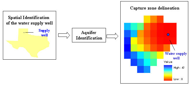
Figure 2. Identification and delineation components for a public water supply
The point source component associates sources with typical areas of contaminated soil and to a list of chemicals emitted from these sources to the environment. The first step in this process is to identify the point sources in the capture zone, which is achieved by spatially intersecting the potential sources coverage with the capture zone. Then each source is related to a list of contaminants and an estimated area, by querying datasets linking the source type with associated properties. Once the capture zone, the spatial locations of the source, the area and the associated contaminants are known, contaminants are diluted and attenuated from their sources to the supply well through the dilution attenuation component of the assessment. Figure 3 illustrates the location of point sources in the capture zone and the tables associated with these sources.
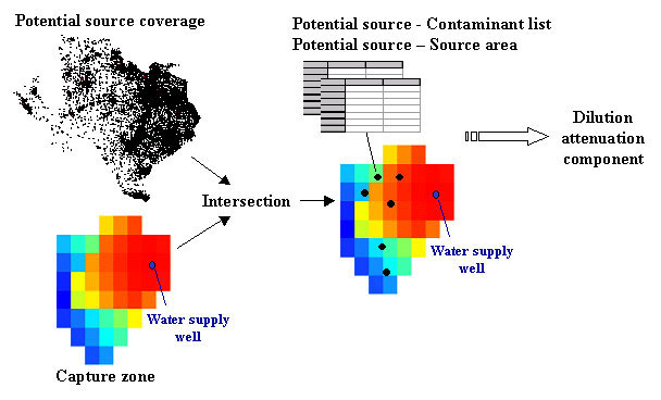
Figure 3. Point Source Component and associated tables
The Tier 2 model is described in the Texas Risk Reduction Program, which is based on a tiered method for assessing contaminant concentrations in groundwater. The tiered methodology begins with the most conservative method suggesting general protective concentration limits in Tier 1 and progresses into more detailed risk assessments in Tiers 2 and 3, which demand site-specific information. The Tier 2 model is a steady state model that calculates dilution of contaminants leaching from soil layers into the water table and the transport and degradation of the constituents in the aquifer. The model incorporates a two-phased approach for describing the movement of contaminants from the soil at the source to the water supply well.
The Tier 2 model is
incorporated in the dilution attenuation component of the susceptibility assessment
to compute the fraction of contaminant reaching a well from each point source
in its contributing area. Implementing this model enables the evaluation of
natural processes and allows natural dilution and attenuation to occur during
contaminant transport in groundwater. This yields a realistic relationship between
the source of contamination and the water quality at the supply well. The first
phase includes the contaminant vertical movement from the soil into the water
table by infiltration and dilution in the aquifer. The second phase is the down
gradient transport in the aquifer from the source of contamination to the water
supply well. Figure 4 shows the two phases of transport represented by the Tier
2 model.
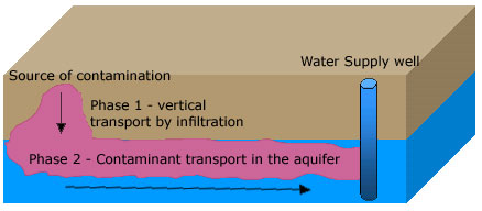
Figure 4. Two phased transport model represented by the Tier 2 equations
The first phase of the model describes leaching of contaminants from contaminated soil into the water table. The Tier 2 equations are derived assuming continuous contaminant emissions into the soil and local equilibrium between the water, air, and particles contained in the soil. Equation 1 is the governing equation used to calculate the ratio between groundwater concentration CGW (g/cm3) and the soil concentration Csoil (g/g-soil). This equation includes a Lateral Dilution Factor (LDF) representing the dilution of constituents entering the aquifer. Equation 1 yields a Dilution Factor (DF), which is the first term required for the Dilution Attenuation Factor,
where ![]() is the soil bulk density (kg/liter),
is the soil bulk density (kg/liter), ![]() the volumetric water content of vadose zone soils (cm3-water/cm3-soil),
the volumetric water content of vadose zone soils (cm3-water/cm3-soil),
![]() the soil water
partition coefficient (cm3-water/g-soil),
the soil water
partition coefficient (cm3-water/g-soil), ![]() the Henry's low constant and
the Henry's low constant and ![]() the volumetric air content of vadose zone soils. L1 and L2
are the thickness of affected soil and the depth from the affected soil's top
to the groundwater table, respectively. In the source water assessment program,
due to lack of more detailed information, the ratio L2/L1
was set equal to one suggesting a conservative approach where the depth of the
contaminated soil (L1) reaches the water table of the aquifer. The
lateral dilution factor is calculated using groundwater velocities in the aquifer
and infiltration rates determined from precipitation rates. In addition, the
LDF is based on the assumption that the constituent leaching from the above
soil is mixed and diluted within an imaginary mixing zone with the dimensions
of Ws and
the volumetric air content of vadose zone soils. L1 and L2
are the thickness of affected soil and the depth from the affected soil's top
to the groundwater table, respectively. In the source water assessment program,
due to lack of more detailed information, the ratio L2/L1
was set equal to one suggesting a conservative approach where the depth of the
contaminated soil (L1) reaches the water table of the aquifer. The
lateral dilution factor is calculated using groundwater velocities in the aquifer
and infiltration rates determined from precipitation rates. In addition, the
LDF is based on the assumption that the constituent leaching from the above
soil is mixed and diluted within an imaginary mixing zone with the dimensions
of Ws and ![]() .
The calculation of the LDF between the contaminated soil and the groundwater
is shown in equation 2,
.
The calculation of the LDF between the contaminated soil and the groundwater
is shown in equation 2,
where ![]() is the groundwater Darcy velocity (cm/year),
is the groundwater Darcy velocity (cm/year), ![]() the net infiltration rate through soil (cm/year),
the net infiltration rate through soil (cm/year), ![]() the ground water mixing zone thickness (meters) and Ws the lateral
width of affected vadose zone in direction of groundwater flow (meters). Figure
4 illustrates the steady state dilution model where a constant flux of contaminant
is introduced into a mixing zone within the aquifer, resulting in a surface
of constant concentration at the end of the mixing zone.
the ground water mixing zone thickness (meters) and Ws the lateral
width of affected vadose zone in direction of groundwater flow (meters). Figure
4 illustrates the steady state dilution model where a constant flux of contaminant
is introduced into a mixing zone within the aquifer, resulting in a surface
of constant concentration at the end of the mixing zone.
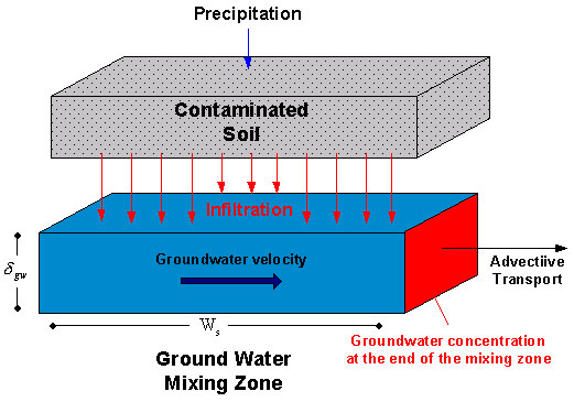
Figure 5. Dilution model yields constant concentration at the end of the mixing zone
The lateral width of contaminated soil is estimated as the width of its source. Within the water assessment program every point source type is associated with an area, the width is then calculated assuming the source of contamination has a rectangle shape. Infiltration rates are calculated depending on the soil type. The Texas risk reduction program specifies three types of soils (sand, silt and clay) used to calculate infiltration.
The second phase of the model describes the transport of the contaminant in the saturated zone of the aquifer from the end of the mixing zone to a water supply well. The model assumes that leaching of the contaminant from the soil layer leads to a well mixed mixing zone, resulting in a rectangular surface at the end of the mixing zone with a constant concentration (calculated in phase 1).
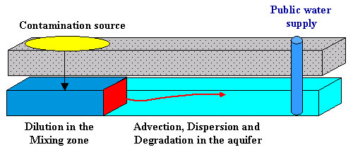
Figure 6. Transport from the end of the mixing zone to the well includes advection dispersion and degradation
Advection, dispersion and decay are incorporated in the model to determine the
effects these processes have on the contaminant concentration at the well. The
time of travel of the contaminant from its source to the water supply well is
integrated into the model through the travel length and the retarded velocity
of the contaminant in the aquifer. The ratio between the concentration at the
end of the mixing zone (CMZ) and the concentration at the well (Cwell)
is the Attenuation Factor (AF). It is calculated using equation 3,
where ![]() is the down gradient flow distance from the source of contamination to the water
supply well (meters),
is the down gradient flow distance from the source of contamination to the water
supply well (meters), ![]() the first order decay constant (day-1),
the first order decay constant (day-1), ![]() the contaminant retarded velocity (meter/day) and W and D are the source width
and depth respectively (meters).
the contaminant retarded velocity (meter/day) and W and D are the source width
and depth respectively (meters). ![]() ,
, ![]() and
and ![]() are the longitudinal transverse and vertical groundwater dispersivities (meters).
are the longitudinal transverse and vertical groundwater dispersivities (meters).
The overall dilution attenuation factor is the final result of the Tier 2 model. The factor is a combination of the two phases of the model described above and results in a ratio between concentrations in contaminated soils and groundwater concentrations at a water supply well. The Dilution Attenuation Factor (DAF) is calculated using equation 4,
![]()
where DF and AF are determined in equations 1 and 3 respectively. Once the DAF is calculated it is incorporated into the susceptibility assessment to demonstrate the effect potential sources in the capture zone may have on the assessed well. Based on the number of sources, the magnitude of contaminants introduced at these sources and the DAF, susceptibility of the water supply to a specific constituent can be determined. For example a certain source with a small dilution attenuation factor suggests that small fractions of contaminants reach the water supply and may indicate a lower susceptibility compared to a well with the same source and a larger dilution attenuation factor.
The application of the Tier 2 model utilizes spatial and non-spatial information assembled in the source water assessment program. These sources are combined together using GIS software to extract values from spatial datasets, representing soil and aquifer data, and relating this information with chemical and potential sources datasets. Datasets of chemical properties were assembled for the dilution attenuation component of the assessment. Due to the number of constituents assessed in the program (~230), the range of the contaminants physical properties and the sensitivity of the assessment to the chemical and physical behavior of the constituents in the environment, it is important to utilize detailed information for each contaminant rather than general groupings or common default values to represent the differentiation between contaminants.
Detailed datasets where developed in the source water assessment program to support the susceptibility assessments. These include a variety of spatial datasets for assessing groundwater as well as surface water for the entire state of Texas. In the groundwater point source attenuation component the following spatial datasets were used to calculate the dilution attenuation factor using the Tier 2 model:
Non Spatial Datasets used in the application include:
The chemical database was established
to support calculations in the dilution attenuation component. It is populated
for all the contaminants assessed in the water assessment program (about 230
contaminants) and is structured in two tables. The first table includes physical
properties such as partitioning coefficients and a chemical type identification.
The second includes a comparison of degradation rates from different sources.
The most conservative degradation rate is used in the calculation (the longest
half life from all sources).
This table is based on a similar
Protective Concentration Level (PCL) table used in the Texas Risk Reduction
Program[4] , which was reviewed,
corrected and populated with missing values. The table contains partitioning
coefficients between the soil phases. It includes such properties as the soil
water partition coefficient (![]() ), the Henry's low constant (
), the Henry's low constant (![]() ) and the soil organic carbon - water partition coefficient (Koc).
The table also includes a general description of the contaminant type. The contaminant
type is used in the Tier 2 application to determine the soil water partition
coefficient (
) and the soil organic carbon - water partition coefficient (Koc).
The table also includes a general description of the contaminant type. The contaminant
type is used in the Tier 2 application to determine the soil water partition
coefficient (![]() ).
).
Degradation and fate processes in
the environment are difficult to model and quantify. These processes are highly
sensitive to a range of site-specific variables, and measurements of degradation
rates reported are highly variable. This makes the task of generalizing the
fate mechanisms into a single representative degradation rate challenging. Because
of these difficulties the most conservative value from all sources included
was used in the attenuation calculation. This approach may result in small attenuation
factors that yield high concentrations at the water supply wells. Such a conservative
method falls within the general framework of susceptibility assessments where,
conservative assumptions are generally applied in the first phase of assessments
followed by more detailed assessment for contaminants exhibiting high susceptibility.
Literature sources such as the Handbook Of Environmental Degradation Rates by Howard et al[5] ,computer models and best professional judgment were used to assemble the database. Computer models that estimate fate and transport are available from a number of sources; the model used in this study is the EPI Suite™ model. This model is a Windows® based interface for physical/chemical property and environmental fate estimation models, developed by the EPA's Office of Pollution Prevention Toxics and Syracuse Research Corporation (SRC) [6]. The model includes half-life estimations in soil, air, water and sediment.
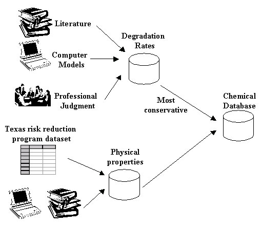
Figure 7. Construction of the chemical database
An application to calculate dilution
attenuation factors from point sources of contamination to water supply wells
was created using ArcGIS and Microsoft Access databases. The ability of ArcGIS
to combine spatial information and tabular datasets and the simple linkage between
it to relational database programs provides an adequate environment to execute
this type of assessments.
The dilution attenuation factor calculation, based on the Tier 2 model, is supported
by the identification, delineation and point source components. Calculations
are done in one Microsoft Access database that assembles all the information
necessary from the spatial and non-spatial datasets. The process is illustrated
in Figure 8. The following spatial and querying procedures are needed to calculate
the dilution attenuation factor from every source in the capture zone of the
water supply well:
Once all the information is assembled into the calculation table, the Tier 2 model application calculates a dilution attenuation factor from each potential source to the assessed water supply well for all contaminants related to the sources in the capture zone.
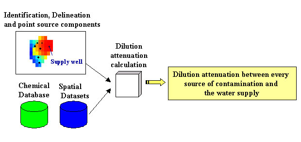
Figure 8. Tier 2 model application diagram
The results of the dilution attenuation
component are numerical values that represent the ratio between contaminants
concentrations in the contaminated soil and their concentration in the groundwater
at the water supply well. The dilution attenuation factors can be applied in
different ways to back calculate target concentrations at the sources or to
conservatively predict groundwater concentrations.
Protective concentrations at the sources can be calculated where target concentrations
or standards exist, by back calculating the concentration from the water supply
to the source of contamination using the dilution attenuation factor. Equation
5 shows the use of DAF to calculate protective concentrations at sources of
contamination,
![]()
where Cpsoc is the concentration at the source of contamination (g/g-soil) and Ctarget is the target concentration at the water supply . As long as concentrations at the source of contamination don't exceed Cpsoc , the target concentration at the water supply will be met.
A different approach may use the dilution attenuation factor to calculate the maximum theoretical concentrations at wells by assuming a theoretical saturation limit or a representative concentration threshold in the contaminated soil, depending on the source type. Then applying the dilution attenuation factor to calculate the maximum theoretical concentration at the well. Theoretical maximum concentrations may be implemented in susceptibility assessments to show the potential influence sources have on water quality at water supplies. By summing the contributions from all sources in the capture zone for a specific contaminant the susceptibility of the water supply can be determined. The calculation of the well concentration based on the cumulative effect from sources of contamination is described by equation 6,
![]()
where i is the number of sources in the contributing zone and DAFi the dilution attenuation factor from sourcei to the assessed well. For example, when applying the DAFs to contaminant threshold at all sources in the capture zone and Cwell yields a lower concentration then the target, it can be concluded that the susceptibility of the well to this contaminant is small. Figure 9 shows these two approaches of dilution attenuation factors implementation.
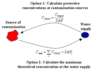
Figure 9. Dilution attenuation factor implementation in susceptibility assessments
An example of the dilution attenuation factor calculation is presented to demonstrate this process. In the example three potential sources of contamination are located in the contributing zone of a water source. These sources are associated with benzene release to soil. Results of the delineation component show that the times of travel from the sources are 5, 25 and 50 years and the flow distances are 100, 500 and 1,000 meters respectively.
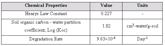
Soil and aquifer properties are presented in table 1 and the physical properties and degradation rate for benzene are presented in table 2. These two tables simulate results from querying the spatial and chemical datasets. An area of 25 square meters is assigned to the sources as a representative area of contaminated soil and an annual precipitation rate of 75 cm/year is assumed at all sources.
Table 1 - Soil and aquifer properties
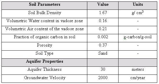
Table 2 - Chemical properties
Applying the dilution attenuation component to these sources yield the following results, presented in table 3.
Table 3 - Results from the dilution attenuation component
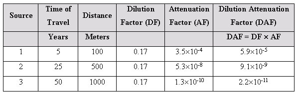
The results in table 3 show the dilution, attenuation and combined dilution attenuation factors. The dilution factor is influenced by the soil and aquifer properties and precipitation. In the example all sources were assigned the same properties and precipitation yielding a constant dilution factor. The attenuation factor decreases as the distance and time of travel increase. Long travel times in the aquifer enable degradation yielding small attenuation factors. These dilution attenuation factors can be implemented into water susceptibility assessments to calculate maximum concentrations at the water supply source or to back calculate protective concentrations at the source of contamination.
The proposed method for calculating dilution attenuation factors and their incorporation in the Texas Source Water Assessment Program is logical and defensible. The Tier 2 model selected to calculate dilution and attenuation of contaminants in the groundwater transport is a well-established leaching and transport model with strong scientific support and applications. The focus here has been to establish a model that provides a numerical link between potential sources of contamination and water supply wells. The model includes the natural processes taking place in the environment between the source of contamination and the well. The numerical connection enables the calculation of expected contaminant concentrations at wells or the backwards calculation of protective concentrations at the potential sources.
The model proposed is executable on a large scale (state), due to extensive dataset construction under the source water assessment program by the USGS and TNRCC, which provides detailed information enabling the use of site-specific detailed models. Another important step was the construction of the chemical database with physical properties and degradation rates, necessary to model contaminants behavior in the environment.
Finally, this method will hopefully contribute to the development of susceptibility assessments by incorporating general site-specific models (such as the tier 2 model), into these large-scale assessments.
[1] USGS Fact Sheet 101-00. July 2000. Overview of the Texas Source Water Assessment Project.
[2] http://www.epa.gov/safewater/pws/pwss.html
[3] Texas Risk Reduction Program. 30 TAC Chapter 350. Tier 2 PCL Equations.
[4] Texas Risk Reduction Program. 30 TAC Chapter 350. Tier 1 PCL Tables
[5] Howard P.H, Boethling S.B, Jarvis W.F, Meylan W.M, Michalenko E.M, Handbook Of Environmental Degradation Rates
[6]
EPA's Office of Pollution Prevention Toxics and Syracuse Research Corporation
(SRC) On-Line EPIWINTM User's Guide (v3.10).