EQPT uses "Habitat Value Units" to asses the ecological quality of selected areas. A Habitat Value Unit is equal to one unit area of pristine or desired habitat. The proximity of waste reduces the value of the habitat. The GIS uses a proximity-based iterative algorithm to aggregate similarly classified waste sites. A variable-size buffering algorithm is then used to approximate the effects of the waste on the environmental quality of the surrounding areas. The user-designated areas are analyzed, and the resulting quality profiles are presented quantitatively in tabular summaries and graphically as grids on vector base maps.
The Ecological Quality Profiling Tool (EQPT) provides an easy-to-use tool for assessing the effects of human activities on the quality of the environment, allows for quick but meaningful assessment of alternatives, and presents the results in effective visual displays. Often, the requisite environmental data exist and the pertinent tools are available to competent GIS analysts, but the transformation of data to information is intricate precluding the analysts from effectively communicating the information extracted from the environmental data.
When designing a GIS tool, one has to be concerned with a proper balance of flexibility and ease of use. Higher flexibility requires users to be more informed and skillful - that is, to have received more documentation and training - to perform the desired task because the tool makes fewer assumptions. The converse is also true: Increased ease of use implies that the user has only to select the appropriate alternative, but he/she is restricted to the encoded set of alternatives. In designing EQPT, we had in mind an ArcView user that is familiar with the basic ArcView functions but is not very familiar with spatial overlays or grid operations.
EQPT is based on the premise that we can assign a value to environmental quality and consequently we can devise a unit of measure for this value. We call this unit the "Habitat Value (HV) " unit. We assign to HV a value of 1.0 per unit area (i.e. acre, hectare) to the Habitat that is perceived to be in a pristine or ideal condition. We assign HV = 0.0 to an area that is a complete ecological catastrophe, e.g., a parking lot. Most habitats have a habitat value 0.0 < HV <1.0.
We also use factors for Element Occurrence Rankings and presence of rare species. Element occurrence rankings are used by many State Heritage programs, and The Nature Conservancy to compare the establish conservation priorities. The rankings are derived by comparing the characteristics of an existing plant community with a defined set of characteristics for a particular community type - the greater the similarity, the higher the rank. Of special importance in this ranking are factors that help to define the "pristineness" of the community, such as the proportion of non-native plants and the presence and quality of surface microbial crusts.
To create the base ecological profile of the existing habitat for the area of interest, we use the following equation:
Base Habitat Value = (wg * grass or understory quality + ws * shrub or overstory quality) * (E.O.Rank) * (rare species) (1)
subject to the constraint wg+ ws = 1 (2)
where:
wg ,ws are weight factors for the grass and shrub contribution to the environmental quality (range 0 .. 1)
E.O.Rank is the Element Occurrence Ranking (1-df1) < factor < (1+ df1)
Rare Species Adjustment factor is (1-df2)< factor < (1+ df2)
df1 and df2 are delta fractions, which are user defined.
For example if the importance of grasses and shrubs is the same, and the value of grasses is set to 1.0 (i.e., ideal), and the value of shrubs is 0.8, and E O Rank = 0.9 and rare species effect is neutral (1.0) then
Base Habitat Value = (0.5 * 1.0 + 0.5 * 0.8) * 0.9 * 1.0 = 0.81
This is calculated for each grid cell within the area of interest. During the calculations, the habitat value is allowed to exceed 1.0, for instance, the presence of a nearby bald eagle nest may result in a rare species factor greater than 1 (e.g., 1.25) which may result in a total habitat value greater than 1.0 if the other factors are also relatively high. However, at the end of the calculations all Base Habitat Values greater than 1.0 are assumed to be of pristine habitat quality and the values are reset to 1.0.
We also assume that the presence of hazardous waste sites will have a degrading effect on the habitat value, and that this effect attenuates with distance from the waste site. EQPT provides three options for calculating this attenuation. These approximations are as follows:
a. Linear 1-y = (a * x) + c (3)
b. Log Linear 1-y = c + a * log10x (4)
c. Quadratic 1-y = (a * x 2) + c (5)
where: y is the habitat value reduction factor (dimensionless)
x is the distance from the hazard site (m) c is the y intercept constant (dimensionless), which may range between 0 and 1 which is the maximum effect that the waste site has on habitat quality a is the slope (1/m), (dimensionless), or (1/m2) for Equation 3, Equation 4, or Equation 5, respectively.
Applying the selected equation (3, 4, or 5) to a grid of waste sites or other hazards results in a Hazard Grid with the greatest hazard levels near the waste sites and minimal hazards beyond a user defined distance.
The approximations and inputs for the base habitat value components and hazard effects should be validated by the user and the parameters determined so as to reflect the same results as the physical process they represent.
The overall habitat value is then calculated as:
where: Hazard Reduction Effect = 1 - y
y is defined by Equation 3 or Equation 4 or Equation 5.
This equation is applied to each unit of area within the area of interest and provides a profile of values that can serve as the basis for characterizing various hazard remediation options of development scenarios.
The steps needed to create an ecological profile are depicted in the EQPT dialog shown in Figure 1 and are as follows:
1. The Habitat Profile frame (first frame of buttons) provides tools to create the Base Habitat Value grid.
a. Invoking the first button, Define Habitat Theme, allows the user to select the desired land cover theme to be used as the basis for the Habitat Value calculations. The Hanford site habitat map shown in Figure 2 is an example of a Habitat theme.
b. The second button, Adjust Habitat Inputs, invokes the dialog shown in Figure 3. Selecting any of the listed options will present an attribute table in edit mode. These attribute tables allow the user to modify the parameters listed in Equation 1.
c. The next button, Determine Species Effect, will draw the species buffers around the species locations and create the species grid.
d. The last button, Create Base Habitat Value Grid, creates the Base Habitat Value grid by combining the species grid with the grid generated from the Habitat theme using Equation 1. An example of the resulting grid is depicted in Figure 4. The more pristine areas are shown in darker colors and higher habitat values.
2. The Area of Interest frame helps the user define the area of interest by creating a new polygon, copying an existing polygon, or editing an existing polygon. The area of interest polygon is then converted to a grid to be used as the limiting area for calculating the Hazard Profile grid and as a mask for the combination of the Base Habitat Value grid and the Hazard profile grid.
3. The Hazard Profile frame of buttons helps the user create the Hazard Profile grid. The Define Waste Sites Theme identifies the spatial characteristics of the various waste sites and for each waste type (e.g., cribs, tanks, burial grounds) or other characteristic (e.g., radioactive, hazardous chemicals, solids, liquids), and defines the distance to the "no effects" level. This distance is then used to define a buffer of influence for each waste type and to consolidate the waste sites that are in close proximity. This consolidation is done to improve the calculation efficiency.
The consolidation algorithm works as follows:
a. Select all the sites of the same waste type.
b. Find the sites that are within a hazard dependent "consolidation distance" from each site. For each site, store in a list all these site IDs and the site to which they are close.
c. Starting with the second site list, go through all the listed sites and see if they are included in any of the previous lists. If, so then consolidate the lists. For example, let the list of lists from step 2 start with
L1 = {1, 3, 22}
L2 = {2, 4, 20}
L3 = {3, 1, 20}
.
Starting with L2, we see that none of the IDs in L2 is in L1; therefore no action is necessary. However, ID 3 in L3 is also in L1; this means that all IDs in L3 will be included in L1, and L3 will be emptied. Now, we have
L1 = {1, 3, 22, 20}
L2 = {2, 4, 20}
.
Obviously L2 should be consolidated with L1, because of site 20. This will happen in the next iteration. Usually three to four iterations are enough to produce a reasonable consolidation pattern.
Site consolidation is performed once for each set of sites and is followed by the creation of a buffer of influence. The Hazard profile grid is then produced by applying one of Equations 3 to 5 for each grid point in the waste buffered areas. An example Hazard Profile grid from the Hanford Site is shown in Figure 5. The locations with higher concentrations of waste are shown in lighter colors in this map. The black areas have "no data" because they are out of the area of interest.
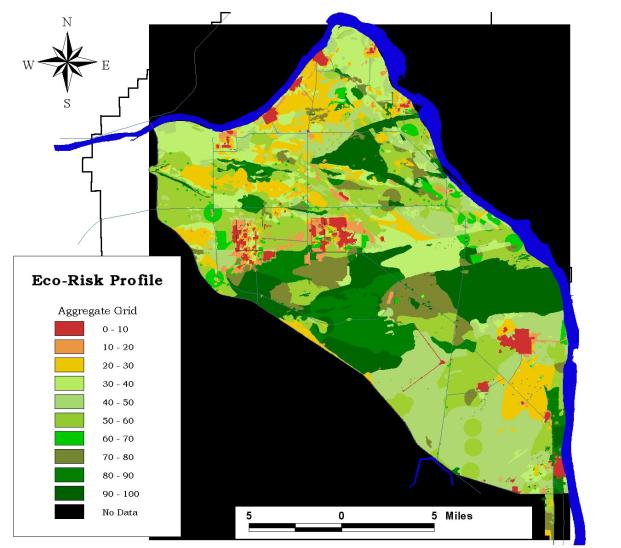
4. The Eco-Q Profile Calculation frame provides buttons to calculate the final profile and summarize the results. Figure 6 depicts an example of final ecological risk profile for an EQPT application at Hanford copied from Reference 1. The red colors indicate areas with lower habitat values due to the influence of hazardous materials. This habitat value grid should be compared to the Base Habitat Value grid, depicted in Figure 4, to determine the influence of the hazardous materials. Again, the darker the green color, the higher the habitat value.
5. The Minimize and Reset buttons are used to hide the Dialog from the screen and reset the values entered so far to their default values.
An example of a summary of habitat value changes for Hanford is shown in Table 1. These values have been calculated using EQPT and are reported in Reference 1.
Table 1. Example Habitat Value Summary for the Hanford Site
| Site Portion | Total Area (ha) | Base Habitat Value (HV/ha) |
Reduction Due to |
% Due to Land Use | Final Habitat Value (HV/ha) | Reduction Due to Hazards (HV/ha) | % Due to Hazards |
| 100 Areas | 5237 | 1988 | 3249 | 62% | 1865 | 123 | 2% |
| 200 Areas | 10243 | 4995 | 5248 | 51% | 4716 | 279 | 3% |
| 300 Area | 1336 | 639 | 697 | 52% | 617 | 22 | 2% |
Total |
16816 | 7622 | 9194 | 55% | 7198 | 424 | 3% |
This paper presented a tool and methodology for assessing environmental/ecological quality for an area of interest based on the use of Habitat Value units. The effects of nearby hazardous waste sites on the habitat value can also be estimated with the EQPT tool. EQPT is easy to use and can help decision making parties determine and communicate the existing or expected environmental quality under different scenarios.
Bilyard, GR, MR Sackchewsky, and S Tzemos. 2002. "Hanford Site Ecological Quality Profile." PNNL-13745. Pacific Northwest National Laboratory, Richland, Washington.
Spyridon Tzemos
Senior Research Scientist
Pacific Northwest National Laboratory
P.O. Box 999, K7-22, Richland, WA 99352
509.375.3683
s.tzemos@pnl.gov
Michael R. Sackschewsky
Senior Research Scientist
Pacific Northwest National Laboratory
P.O. Box 999, K6-85, Richland, WA 99352
509.376.2554
michael. sackschewsky@pnl.gov
Gordon R. Bilyard
Technical Group Manager
Pacific Northwest National Laboratory
P.O. Box 999, K3-54, Richland, WA 99352
509.372.4219
gordon.bilyard@pnl.gov