From Outcrop Observations to Geologic Reservoir Models using Esri
Software
Marieke Dechesne, Jim Borer, Donna Anderson
Slope and Basin Consortium
Department
of Geology and Geological Engineering
Colorado
School of Mines
Golden, CO
80401
ABSTRACT
The gap between geologic mapping and geologic reservoir models can be bridged
with Esri software. Data are collected in the field by a team of geologists
using handheld GPS, paper maps, and ArcPad. After collection, the gps points
are transferred to an ArcView database. In the office, data are interpreted and
analyzed using ArcView Spatial and ArcView 3D Analyst. Map layouts are
produced, and the shapefiles are exported to geologic reservoir modeling
packages, such as Petra, Petrel or GOCAD. The ArcView database is being
integrated with a general relational database containing both spatial,
geologic, interpreted, petrophysical, and reservoir information.
Mapping with GIS has become an important step in the workflow to go from outcrop observations to reservoir models, both in storing and transferring geospatial information and in developing a database to store large amounts of detailed data.
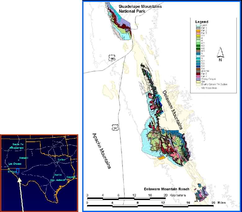
The SBC currently studies outcrops of the Brushy Canyon Formation (Permian, Guadalupian) in the Delaware Mountains of West Texas (see figure 1). The outcrop belt covers 245 km2, ranging from Guadalupe Mountains National Park to just north of Van Horn, Texas.
Figure 1. Overview of study area location. The outline of the Brushy Canyon Fm. is shown in light yellow. The currently mapped units are colored.
The Brushy Canyon Formation is a 350 meter thick interval of marine sandstone and siltstone deposited in water depths ranging from 200-500 meters. The 55 km long outcrop belt provides an oblique-dip view of a slope-to-basin depositional profile (see figure 2) and is studied at a varying detail ranging from centimeters (thin sections) to 100’s of meters (stratigraphic sequences). The Brushy Canyon Formation is subdivided into nine internal units, which record the growth and retreat of individual submarine fans. These “fan-scale” (5th-order) depositional cycles range from 20-70 meters in thickness and are bounded by regionally mappable siltstone packages that record periods of fan abandonment.
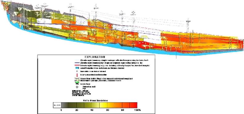
Figure 2. Regional, oblique-dip cross section for the nine fan units. Net:gross variations over the interval are indicated by varying colors from green (low % sand) to red (high % sand). Cross section length is 55 km.
Reservoir heterogeneity is controlled by the vertical and lateral changes within, and between, individual “fan-scale” cycles. For each fan, the character and lateral extent of slump scars, channels, lobes, inter-lobes, and siltstones are mapped for multiple small-scale time slices (10-20 m thick, 6th-order depositional cycles). With this detailed information, several stratigraphic and sedimentologic models are constructed to explain changes in deep-water fans through time and space. The strength of the Brushy Canyon as an analog lies in both the stratigraphic and paleogeographic context provided in the outcrop belt. Temporal changes in net:gross, facies and reservoir architecture are documented at local and regional scales in both depositional strike and dip directions.
Detailed dimensional architecture data is collected by decimeter-scale mapping on photo panels of canyon walls. From interpreted photo panels, measurements are taken on the dimensions, facies fill and spatial relationships of a hierarchy (i.e., channels, channel complexes and conduits) of architectural elements (channels, lobes, wedges and siltstone sheets).
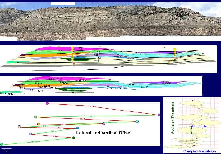
Figure 3. Example of photopanel interpretations and measurements.
The photo panel locations are mapped as an Arcview shapefile, so it is easy to link the measured dimensions to a location in the study area. The measurements are an important input parameter for reservoir models. The outcrop dimensional data can be applied to a broad range of subsurface reservoir problems using the proper stratigraphic and paleogeographic analog and adjusting and normalizing the data based on an understanding of the depositional processes. Parts of the Brushy dataset have been applied as an analog for reservoirs in the Permian Basin (West-Texas), Gulf of Mexico, Offshore West Africa, and the North Sea.
A primary goal of the SBC is to develop techniques for building better deterministic and stochastic flow models of deep-water sandstone reservoirs. Outcrop-based reservoir models are built by combining petrophysical information (porosity and permeability) with maps, cross sections and measured sections. The outcrop dataset allows for the construction of highly deterministic models that can be used as a base case for testing models built from sparse datasets using various stochastic algorithms. Outcrop isopach, net sand and channel trend maps are highly deterministic given the three dimensional nature of the outcrop, extensive photo panel coverage and large number of measured sections. Geologic modeling rules are being developed and tested for their ability to adequately represent deep-water sandstone reservoir heterogeneity as measured by dynamic fluid flow response.
Software used includes ArcView 3.2a, but also ArcInfo 8.2 and ArcPad 6.0. Importing arcview shapefiles and/or surface grids into modeling software packages (IRAP RMS, Petrel, GoCad and Petra) has streamlined reservoir model construction. A custom RSI-ENVI program has been developed in IDL to ortho-rectify images
Three overlapping domains describe the past, present and future of SBC GIS projects. Past GIS efforts involved the conversion of the project from CAD based mapping to detailed ArcView mapping using handheld GPS data. Current GIS utilization involves the use of shapefiles in the creation of outcrop-based “subsurface” datasets and reservoir models. Future GIS work includes the construction of a relational database that allows users to help the user properly query and filter outcrop analog data and to take virtual field trips by hotlinks to photgraphs. Recent and future work also includes the integration of high-resolution LIDAR digitial elevation models for draping and ortho-rectifying photo panel interpretations for geospatial measurements and input into modeling software.
In previous years, SBC geologic mapping was done without GPS units and maps were created in CAD drawing package (Canvas 5-7, Deneba) set up in drawing units rather than georeferenced map units. Drawing objects had no attributes and were not stored in a database. Exporting map data to other software packages involved an inefficient re-digitization step. With the release of the GPS signal and our need for more accurate mapping, the SBC shifted 1.5 years ago to using Esri GIS software. Advantages are a better data organization, attribute storage, possibilities for gridding and contouring map data, 3D projections and easy import\export to geologic modeling packages. Because initial mapping was done in drawing units on non-rectified topographic scans, the conversion to ArcView through dxf format was time consuming and not accurate enough for our purpose.
Mapping an outcrop belt such as the Delaware Mountains starts at identifying the stratigraphic (geologic) units to map. One way to do that is to measure detailed stratigraphic sections, describing every sand or siltstone bed in a vertical succession for grainsize, sorting and sedimentary structures. Part of our field mapping technique is to take GPS points at every significant siltstone break at measured sections. The siltstone intervals represent breaks in sedimentation, which are often internal or external submarine fan boundaries, and are important reservoir flow boundaries. Between measured sections, major siltstone intervals are walked out and extra GPS points added to define geologic map (cycle) boundaries. Currently 24 siltstone-bounded units are mapped and include both fan-scale and sub fan-scale layers.In some detailed study areas individual siltstones are mapped as separate units, doubling the layers mapped. GPS measurements are also used to map faults and the location and size of sediment bodies such as channels and/or channel complexes (figure 4).
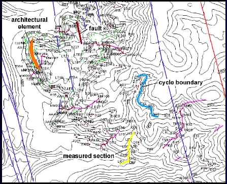
Figure 4. Example of elements mapped from GPS points: measured sections (pink and yellow), cycle boundaries (light blue), architectural elements (orange), photopanels (dark blue) and faults (red).
The SBC uses six Garmin ETREX Summit GPS units, with an accuracy ranging from 2-5 meters (in x,y positions). The units are generic hiking models rather than differential GPS. For the purpose of our mapping, with all errors (accuracy of maps, accuracy of interpretations, size of features) taken into account, the GPS accuracy is considered sufficient enough for its cost. Data points are downloaded through MapSource (Garmin), and saved as textfiles. Then they are converted to shapefiles in ArcView 3.2a via the AVGarmin extension that was downloaded from the Esri ArcScripts website (http://arcscripts.Esri.com/details.asp?dbid=11515 , author: California Department of Fish and Game, Isaac Oshima, 2001). Once the GPS points are imported to shapefiles, they are used to make polylines for measured sections or polygons to define geologic map units (see figures 5 and 6). Currently we are also doing tests with ArcPad 6.0 (NMEA supported), on a Compaq IPAQ and Etrex Summits, to digitally map channel trends and geologic boundaries in the field.
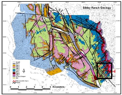
Figure 5. Overview of fan scale mapping.
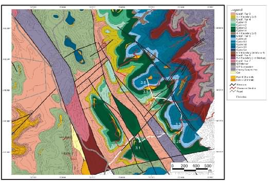
Figure 6. Overview of cycle scale mapping.
In addition to basic geologic mapping, ArcView is also an essential tool for getting deterministic outcrop data into subsurface petroleum reservoir modeling software packages. Channel trend maps (figure 7) facilitate the construction of isopach and net sand maps and the creation of channels in reservoir modeling software (Roxar-IRAP RMS and Technoguide-Petrel).
Figure 7. 3D display in ArcView of channel trend maps.
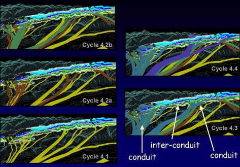
Figure 7. 3D display in ArcView of channel trend maps.
Isopach and net sand maps are constructed by hand editing computer contoured maps of measured section data, using channel trend overlays and incorporating 2D photo panel information. ArcView shapefile of channel trends are converted to a channel isopach and Z value map pairs that are gridded.
Isopach and net sand maps are constructed by hand editing computer contoured maps of measured section data, using channel trend overlays and incorporating 2D photo panel information. ArcView shapefile of channel trends are converted to a channel isopach and Z value map pairs that are gridded.
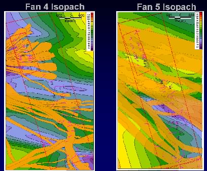
Figure 8. Example of isopach trends with overlying channel trend shapefiles in Petra.
Math operations on the gridded surfaces allow multiple channels to be accurately placed into the model space as the difference between two surfaces offset from a third surface. Although ArcView can facilitate the placement of channels, surface based channel models are inefficient (hundreds of surfaces), inaccurate and difficult to edit.
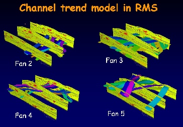
Figure 9. Channel trend models in RMS.
More recent models are built using topologic object-based modeling software (Tsurf-GoCad). ArcView shapefiles of outcrop channel trends and cross sectional areas are easily imported into GoCad (http://www.ensg.inpl-nancy.fr/GOCAD/ or http://www.t-surf.com/products/gocad/). Three-dimensional editable channel objects are then created in GoCad using the channel trends and cross-section data as a skeleton around which a skin is interpolated (figure 10).
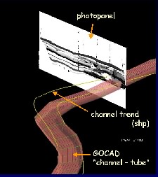
Figure 10. GOCAD Channel-tube created by using the outline of the ArcView channel trend shapefile. The photopanel with interpretations are positioned in the model by using the photomosaic shapefile.
The need to treat measured section paths as deviated wells is another difficult issue that is solved using a combination of ArcView and GoCad. An ArcView polyline shapefile of measured section paths is constructed from GPS data and imported into GoCad. In GoCad, z-values are added to the section path by common point extraction from the USGS 30 m DEM (figure 11).
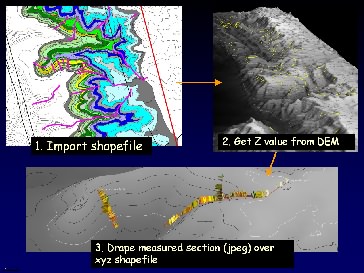
Figure 11. Work flow for importing shapefiles into GOCAD. 1) Import the measured section shapefile. 2) Drape shapefile over 30m USGS DEM. 3) Drape *.jpg file of measured section over the measured section shapefile to create a “deviated well” path.
The 3D paths are then hand edited so that the total thickness of the path corresponds exactly with the measured thickness. Digitized measured section data (facies, grainsize and outcrop gammaray) are draped onto the 3D section paths and offset to the correct depth creating a deviated “well” that is used to condition subsurface petrophysical models. Some measured sections span over 0.5 km map distance and therefore treating sections as a vertical well with a midpoint location is inadequate for the accurate placement and extrapolation of geologic features such as channels, facies, petrophysical properties (figure 12).
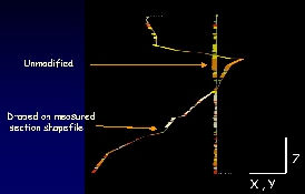
Figure 12. Illustration of the difference between a regular well and a deviated well . Note the difference in X and Y directions. By using a straight well an error of up to 0.5 km can be easily introduced to the model.
Recently a start has been made to create a relational database between the spatial (GIS) data and detailed photo panel dimensional measurements and rock property data (figure 13).
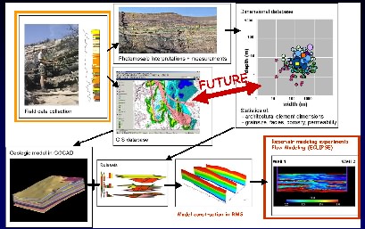
Figure 13. Summary of the SBC workflow from outcrop to reservoir model.
This extensive database will be accessible to our sponsors over the internet through a geospatial interface in ArcIMS (figure 14). Cross queries by paleogeographic region, geologic unit (fan) or specific photo-panel or measured section will provide an easy and effective way to mine the extensive dimensional data collected for each canyon wall. Cross referenced graphical hyperlinks of maps, photo panels, cross sections, measured section, facies photos and models will provide a virtual fieldtrip, which will allow users to choose the proper analog within the Brushy and/or future datasets.
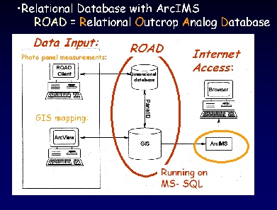
Figure 14. The relational dimensional database and GIS mapping will be linked in the near future. The data can be queried and displayed over the internet by ArcIMS.
Future plans may also include the acquisition of a LIDAR system (figure 15). Several field tests have indicated the advantages and costs of creating highly detailed (3-10 cm resolution) DEMs of our study area (figure 16). With the high-resolution DEMs (and the use of a special application build in IDL for use with RSI-ENVI), the distortion present in photo panels of canyon walls can be rectified in a more accurate and automated fashion than by hand (figure 17, figure 18). This is an important enhancement in our workflow that will ultimately allow us to fill the database with accurate dimensional measurements of the mapped architectural elements and facies. Georeferenced LIDAR point cloud data can also be directly brought in and manipulated in GoCad to help constrain the placement of geologic objects. ArcGIS will likely be part of the workflow to georeference and fully utilize the LIDAR data.
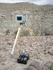
Figure 15. Ground based LIDAR system (ILRIS 3D, from Optech) operating in the Delaware Mountains.
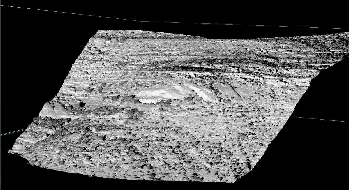
Figure 16. Detailed (3-5 cm) DEM acquired with the ILRIS 3D.
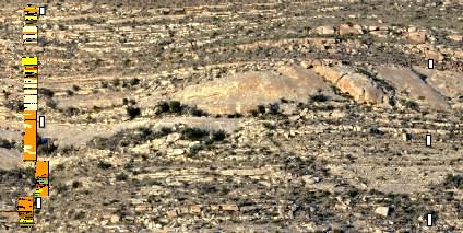
Figure 17. Original photopanel, with distortion. Bars indicate vertical scale before ortho rectification.
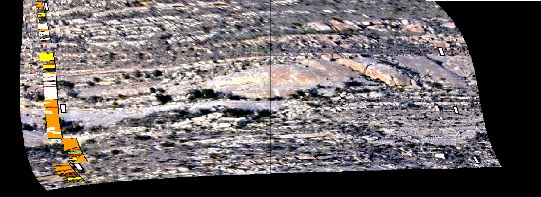
Figure 18. Ortho rectified image (in the ENVI-photostrat IDL application), note the different size in the scalebars, indicating the change in scale (compare figure 17).
We would like to thank all sponsors of the Slope and Basin Consortium (BP, BHP, Conoco Inc, Exxon-Mobil, Kerr-McGee Oil Company, Marathon Oil Company, Nexen, PetroBras, Philips Petroleum Company, Statoil, Total-Fina-Elf, Texaco Exploration and Production Inc. Unocal Corperation, Roxar, Landmark, RC2 Research Systems Inc. RSI Inc, IReservoir) for their support and feedback. Also all staff and students of the SBC are thanked for their help and input in this GIS project.