ESTIMATION OF
INSTANTANEOUS UNIT HYDROGRAPH WITH
Nurünnisa Usul and
Abstract
Determination of the unit hydrograph of a basin
is very important for the design of hydraulic structures. When there are observed
rainfall-runoff data for the storms they are obtained by using these data, but
when there are no observed data they are obtained by using synthetic unit
hydrograph methods. In this study one such method is used together with
Geographical Information Systems techniques. Application of
Key words: Instantaneous Unit Hydrograph,
1. INTRODUCTION
Main consideration of hydrology is the
rainfall-runoff relationship of a watershed. The response of a watershed to
rainfall is observed as the runoff at the basin outlet. For the gauged basins
this is recorded as hydrograph (discharge vs. time graph). The unit hydrograph
of the basin is the surface runoff hydrograph caused by a unit excess rainfall
distributed uniformly over the area, and its determination is significant in
hydrology. For gauged basins unit hydrographs are determined from observed
storm data; hyetographs and corresponding hydrographs. For the ungauged basins there are several
techniques for derivation of unit hydrographs synthetically.
Time of concentration, Tc, is the period of time that it takes for flow from the remotest point in the basin to reach the watershed outlet. In this study the Soil Conservation Service (SCS) lag equation is used to determine Tc value. SCS equation requires main channel length, average Curve Number and slope of the basin, which are evaluated by the tools of GIS. As GIS softwares, Arc/Info (Esri, 1999), ArcView (Esri, 1998) and Watershed Delineator extension (Esri, 1997) of Environmental Systems Research Institute are used in this study.
Reservoir storage coefficient, R, is the second parameter of the methodology reflecting the storage effects of the stream channels. R is computed graphically from an observed storm hydrograph of the basin. Then the coefficient is used to rout the translation hydrograph to the basin outlet.
The time-area histogram represents the area of the basin contributing to the flow at the basin outlet at any given time after the application of a unit excess rainfall. Reflecting the shape and drainage properties of the basin, it is the most important parameter for derivation of the translation hydrograph. The Digital Elevation Model (DEM) of the basin, which is the 10x10 meter cell sized grids having elevation values, is used for this purpose. First travel distance of each cell to the outlet is determined by estimating cell flowlengths. Then travel distance of each cell to the determined outlet (in time units) is derived from cell flowlengths. Then the time-area graph of the basin is determined. After instantaneously applying a unit excess rainfall over the basin, the translation hydrograph is derived from the time-area graph. The translation hydrograph, which reflects the travel time of runoff to outlet, is then routed by linear reservoir and Instantaneous Unit Hydrograph (IUH) of the basin is determined.
Instantaneous unit hydrograph is the result of a unit depth of rainfall occurred in an infinitely small time interval over the basin. Since the duration of rainfall is assumed as zero, shape of the hydrograph depends only on the basin characteristics.
2. STUDY AREA
Study area is the upstream part of
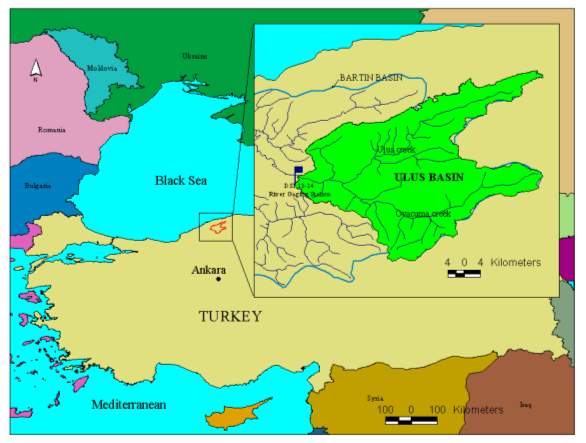
Figure 1. Location of Ulus Basin
3. ESTIMATION OF CURVE NUMBER
The Runoff Curve Number method, developed by U.S. Soil Conservation Service (SCS) is a widely used methodology for understanding the response of the basin to rainfall. The Curve Number (CN) values ranging from 40 to 100 reflect the land condition as a function of soil type, land use, vegetal cover and soil moisture condition of the basin. SCS has published guidelines for estimating CN values of various areas depending on the listed parameters (ASCE, 1996).
3.1. Soil and Landuse Maps
Soil and landuse maps of the area are obtained in hardcopy form. Five soil and landuse map sheets covered the whole basin. These hardcopy maps are first scanned by A0 drum scanner and stored as “jpg” image files. Then they are geocoded with reference to the 1:100000 scaled hardcopy map sheets of the area. Finally by on screen digitizing, soil and landuse maps are obtained in digital format.
After digitizing the soil and landuse maps, the information on the hardcopy map sheets are placed in the prepared database. A four-column table is created, columns having names: MSG for Main Soil Group, Landuse, HSG for Hydrologic Soil Group and CN for Curve Number. Information about main soil group and landuse types is determined from hardcopy map sheets. Hydrologic soil group values are obtained from the tables prepared by General Directorate of Rural Services of Turkey. These values represent HSG as a function of soil type. Then the Curve Number value of each area in the map is determined from SCS tables.
3.2. Average CN value of the basin
After transforming the digital soil and landuse maps to shapefile format, it is clipped
with the digitized basin boundary. The obtained landuse map of
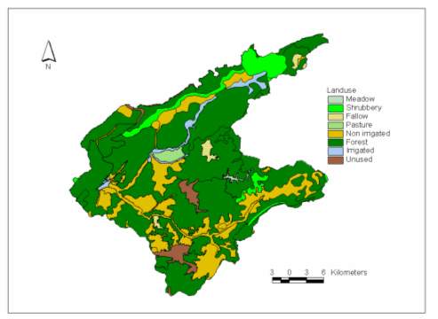
Figure 2. Landuse types in Ulus Basin
Moreover, it is observed that most of the basin area is covered with forests. Only a small percent of the area is used for farming and these are around the main channels (Ulus and Ova Creeks). Hydrological soil group of the basin is mainly C type representing less permeable soils having low infiltration rates when thoroughly wetted.
4.
APPLICATION
OF CLARK
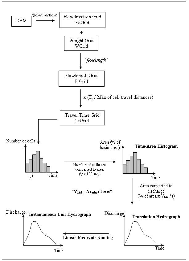
Figure 3. Flowchart of the methodology
4.1. Time of Concentration
Time of concentration is the time required for excess rainfall to travel from the most remote point of the basin to the outlet. At the end of this time, entire basin will be contributing to the flow at the outlet. In literature, several equations are available for calculation of time of concentration (ASCE, 1996). After considering the availability of parameters the following SCS equation is selected for this study.
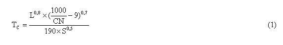
Where, Tc
is the time of concentration in minutes, L is the longest flow path of
the basin in feet, CN is the average Curve Number value of the watershed
and S is the average watershed slope. Longest flow path is the maximum
value of Flowlength Grid (FlGrid).
As described in the next section, the FlGrid represents
travel distance of each cell in the basin to the outlet. In this study two FlGrids are calculated: for weight condition and no weight
condition. Average CN value of the basin was determined as 76. Average
watershed slope is derived from slope grid (SGrid) of
the basin, which is obtained from DEM. After clipping SGrid
with the watershed boundary, mean value of the clipped SGrid
is determined as 0.3327. By inserting these values in Equation 1, the time of
concentration value of
4.2. Storage Attenuation Coefficient
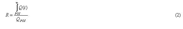
The storage attenuation coefficient, which represents the storage effect of stream channel, is calculated from an observed flood hydrograph of the basin. As described in Figure 4, R is graphically computed as the ratio of volume under the hydrograph after the second inflection point (under recession curve) to the value of the flow at the point of inflection (POI) (HEC, 1982).
The observed flood hydrograph of
the basin is obtained from State Hydraulic Works of Turkey; it is the storm,
which occurred on
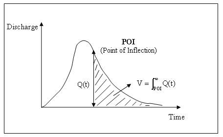
Figure 4. Calculation of storage attenuation coefficient (R)
4.3. Time Area Histogram
The area of the basin is divided into travel time zones. Each zone represents the part of basin, which drains the unit excess rainfall to the outlet at a certain time interval. The plot of these areas with respect to corresponding time intervals gives the time-area histogram of the basin. It is the most important parameter of the methodology, since it reflects the runoff response of the basin to the rainfall at the outlet.
The 10 x 10 m cell sized digital elevation model of the basin is used for determination of time-area histogram. For this purpose, the direction of flow from each cell is found first. Than by tracing the flowdirection, travel distance of flow from each cell to the basin outlet is calculated. These distances are turned to travel time values. Finally by converting the number of cells to area, the time-area histogram is derived. These steps are explained in the following sections.
4.3.1. Flowlength Grid
As described in Figure 3, to
obtain the time-area graph of
In a square grid environment, each grid cell is surrounded by eight cells. As described in Figure 5, direction of flow from a cell can be represented by assigning a number representing one of the eight directions. Using GIS tools flowdirection value of each cell in the basin is calculated from the DEM of the basin then a grid containing these values is obtained and named as flowdirection grid, FdGrid.
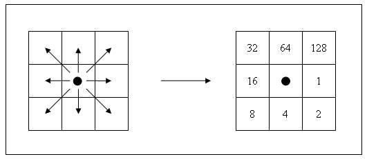
Figure 5. Flowdirections
Velocity of flow in an area will differ depending on the topography and landuse conditions. Water will move slowly in a mild slope or over a dense pasture area and faster on a bare land. To represent the impedance or resistance of the cell to the flow, a grid can be prepared. The value at each cell in this grid represents the resistance per unit distance to flow through the cell or weight of that cell. The grid containing values which represent the weight of each cell is named as weight grid (WGrid).
After determining the direction of flow from a cell to one of the neighboring eight cells, slope distance between centerlines of these cells is calculated. Then this distance is multiplied by the WGrid value of the first cell to obtain the weighted distance value between these two cells. Finally the FlGrid cell values are obtained by summing these values along the flow path to the outlet for each cell. As mentioned before, in calculation of FlGrid, the usage of WGrid is optional. In this study in addition to weight grid condition, no weight grid condition is also analyzed. For the former one, a weight grid is prepared as described below and used with the flowdirection grid for calculation of flowlength grid. For the latter one, only the flowdirection grid is used in calculation, where the weight of each cell is accepted as the same and equal to 1.
4.3.2. Weight Grid: From Application of Manning’s
Equation for
Manning’s equation (Equation 3), which is frequently used in fluid mechanics, is also applicable to overland flow. In this study Manning’s velocity equation is used to compute the velocity grid named as VGrid. The grid represents the velocity of flow in each cell. To obtain a velocity grid, all the parameters of the equation (n, R and S) are prepared in the form of grids and inserted into Equation 3 as given in Equation 4.
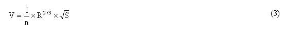
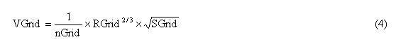
The grid, which contains values representing Manning’s roughness, is named as nGrid and determined as a function of vegetation type or landuse. The slope grid of the basin is derived from DEM of the area and named as SGrid. For open channels, hydraulic radius is the ratio of flow area to wetted perimeter, but for overland flow it is accepted as the depth of flow. The grid containing hydraulic radius values for streams and depth of flow for the other parts of the basin is named as RGrid. The Manning’s equation gives VGrid values representing velocity of flow in each cell.
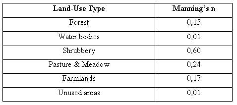
Manning’s roughness coefficient for overland flow
Roughness coefficient is the
most significant parameter of the Manning’s equation. It depends on vegetation
cover or landuse type of the area. Tables giving n
values for different landuse types are available in
the literature. Roughness values for
Table 1. Manning's roughness coefficients for landuse types
Hydraulic Radius for streams and overland flow
The second parameter of the Manning’s equation is the hydraulic radius value. For open channels hydraulic radius is calculated from the ratio of flow area to wetted perimeter of the channel. But in order to obtain the velocity grid of the whole basin, in addition to stream channels, hydraulic radius values of the overland areas must also be assigned. A grid named as RGrid is prepared representing hydraulic radius value of each cell in the basin. In this study hydraulic radius in Manning’s equation is considered for two cases.
a) Overland flow: In open channel hydraulics it is known that hydraulic radius of wide rectangular channels can be accepted as the depth of flow. The cells in the RGrid that are not forming stream channels are accepted as overland flow areas. A thin layer of flow will occur on overland flow areas, where these cells can be treated as wide channels. Since a unit hydrograph is to be evaluated at the end of the study a surface runoff depth of 1mm (0,001 m) is taken as the flow depth.
b) Streams: Hydraulic radius of open channels is
calculated from geometry of the channel. But in a grid based representation of
the topography it is hard to estimate the cells forming stream beds. The flowaccumulation grid, which is
named as FaGrid, of the
basin is used for this purpose. FaGrid
is computed from the FdGrid
that is obtained from DEM of the basin. Any cell value of FaGrid indicates the number of the cells giving all
their surface waters to that cell. Than the river network is extracted by
accepting the cells as stream beds which have an FaGrid
value greater than a predefined threshold value, which is accepted as 1000 in
this study (Usul, 2002). On
a DEM having 10x10 m size grids, 1000 cells represent a stream initiation area
of 0.10 km2 and the cells having a drainage area greater than 0.10
km2 constitute the stream network. After defining the streams,
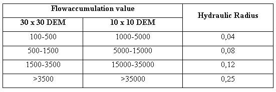
hydraulic radius values of these cells are estimated. In a similar study (Fleckenstein
1998) that utilizes Manning’s equation on a 30x30 m resolution, R values given
in Table 2, are used. The stream initiation threshold value used in that study
is 100 cells. Then, as described in Table 2 the number of cells forming streams
are ordered in four groups according to their flowaccumulation values, and a single hydraulic
radius value is assigned to each group. On the 30x30 m DEM, 100 cells represent
a stream initiation area of 0.09 km2. Accepting this study value
close enough to the value selected for
Table 2. Hydraulic radius values
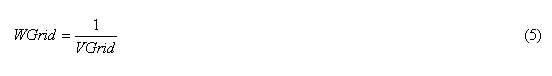
After deriving slope of the basin the velocity grid (VGrid) is obtained using Manning’s equation (Equation 4). The VGrid represents the flow velocity in each cell of the basin, which is used to compute weight grid. The weight grid used in this study is computed as the inverse of VGrid and named as WGrid (Equation 5). Finally this weight grid (WGrid) is used to compute FlGrid of the basin as described previously.
FlGrid of the basin is then determined from the input grids of FdGrid and WGrid.
4.3.3. Travel Time Grid
After computing the travel distance of each cell (FlGrid), the next step is calculating the travel time values. The maximum value of the FlGrid belongs to the remotest cell of the basin to the outlet. Travel time of flow from that cell to outlet gives the time of concentration value of the basin. Equation 6 is used to prorate the values of FlGrid and to convert it to time values (Kull and Feldman, 1998). The travel time grid of the basin is then determined from Equation 6 and named as TtGrid.
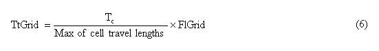
In Equation 6 “maximum of the cell travel lengths” is the maximum value of FlGrid and Tc is the time of concentration value of the basin. Two travel time grids are calculated using the two flowlength grids and Equation 6, for weight grid and no weight grid conditions.
The third
parameter of the
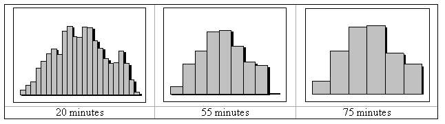
Figure 6. Histograms of travel time grid with different time intervals for no weight grid condition
IUH of
the basin will be derived if the selected time interval is infinitely small.
Practically it is impossible to obtain the histogram of TtGrid with infinitely small time interval. So the
smallest possible time interval is selected to apply the
Histogram of TtGrid has time values on the abscissa and number of cells on the ordinate. The time-area histogram of the basin is calculated from histogram of TtGrid by converting number of cells to area (100 m2 for 10x10 m grid). The time area graphs of Ulus basin is obtained for weight grid (Figure 7) and no weight grid conditions.
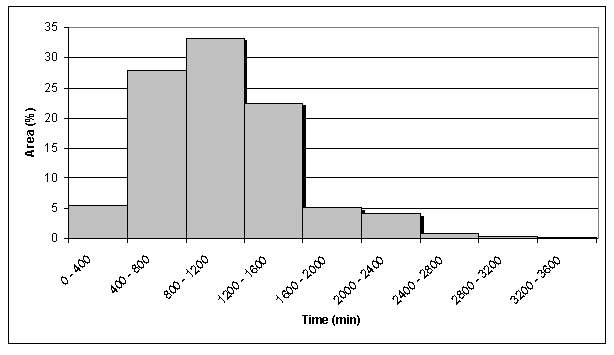
Figure 7. Time-area histogram of Ulus Basin for weight grid condition
4.4. Translation Hydrograph
After
determining the three parameters of
After instantaneous application of unit rainfall, total volume of water that will be observed at the basin outlet is determined by multiplying basin area (955 km2) with the depth of precipitation (1 mm). Then from the time-area histogram of the basin, percentage of total volume contributing to the flow at the outlet in each time interval is calculated. Volumes are then converted to discharges for corresponding time intervals. Finally by plotting these values at the mid values of time intervals the translation hydrograph is determined. Similar to time area graph two translation hydrographs are obtained, one for weight grid condition (Figure 8) and another for no weight grid condition.
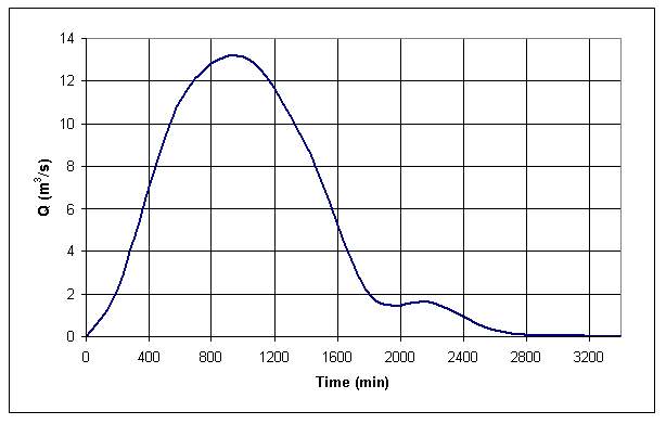
Figure 8. The translation hydrograph of Ulus Basin for weight grid condition
4.5. Linear Reservoir Routing
As previously mentioned the instantaneous unit excess rainfall is conveyed to the basin outlet by two components: a translation hydrograph and linear reservoir routing. The translation hydrograph represents the rainfall-runoff relationship of the basin by means of surface flow only. The effect of stream channel storage on the hydrograph is reflected by linear reservoir routing. The translation hydrograph obtained in the previous section is routed by Equation 7 (HEC, 2000).
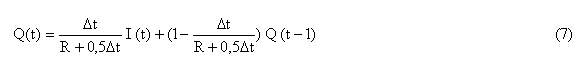
In Equation 7, I(t) is the calculated translation hydrograph, R is the storage attenuation coefficient and Dt is the selected time interval for routing. Q(t) which is obtained after routing is the instantaneous unit hydrograph of the basin. The routing process is continued till an excess flow depth of 1 mm is obtained under the hydrograph. Instantaneous Unit Hydrograph of Ulus Basin, is obtained for weight grid and no weight grid conditions separately.
5. CONCLUSION
In this study two Instantaneous Unit Hydrographs are obtained. First a weight grid is prepared and used as input to derive time area histogram of the basin. The weight grid reflects the resistance of each cell in the basin to flow according to topographic and vegetal cover conditions. Secondly no weight grid case is used where all the cells in the DEM of the basin are assumed to have equal resistance to the flow.
Then these hydrographs are compared with the
observed unit hydrograph of the basin, which is determined in another study (Usul,
2002). Since the observed unit hydrograph
is for 60 minutes duration, same duration unit hydrographs are also determined
using these IUHs. The three
unit hydrographs (observed, Clark-weight,
Table 3. Properties for unit hydrographs
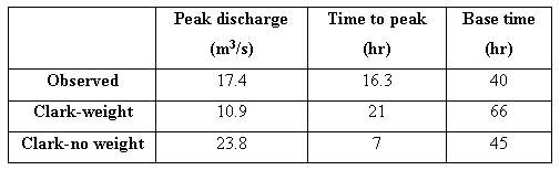
As demonstrated in Figure 9 the
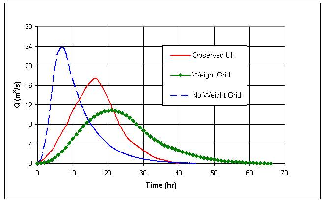
Figure 9. Synthetic and observed 1 hour duration unit hydrographs of Ulus Basin
In the second case a weight grid is prepared to represent topographic and vegetal cover conditions of the basin. But use of weight grid results a late coming and lower peak discharge than the peak of observed unit hydrograph. The weight grid, which is developed from Manning’s equation, results a high retardation in the flow. So discharge development occurred slowly and a late hydrograph peak is formed. So, it is concluded that resistance effect of Manning’s equation on the flow is more than the actual basin conditions. The most significant parameter of the Manning’s equation is the roughness coefficient. The hardcopy soil and landuse maps used to obtain the coefficients were old, therefore they may not reflect the actual land conditions. After considering the significant difference in the two synthetic unit hydrographs, it is also concluded that use of weight grid in this methodology is very important and a revised weight grid may fix the discrepancies in the result.
6. REFERENCES
ASCE, 1996: American Society of Civil Engineers
Hydrology Handbook, 2nd Edition,
Clark, C.D., 1945: Storage and the Unit Hydrograph, ASCE Transactions, 110, p. 1419-1446.
Esri, 1997: ArcView
Watershed Delineator User’s Manual, Esri
Esri, 1998: ArcView
User’s Manual, Esri
Esri, 1999: Arc/Info User’s Manual, Esri
Fleckenstein, J., 1998: Using GIS to
derive Velocity Fields and Travel Times to Route Excess Rainfall in a
Small-Scale Watershed,
HEC, 1982: Hydrologic Engineering Center: HEC-1
Training document No.15, U.S. Army Corps of Engineers,
HEC, 2000: Hydrologic Engineering Center HEC-HMS
User’s Manual,
Kull, D. W. and Feldman, A. D., 1998: Evaluation of Clark’s Unit Graph Method to Hydrologic Engineering Center Spatially Distributed Runoff, Journal of Hydrologic Engineering.
Usul, N., 2002: A Pilot Project for
Flood Analysis by Integration of Hydrologic-Hydraulic Models and Geographic
Information Systems (in Turkish), METU,
Authors:
Nurünnisa Usul
METU, Civil Engineering Dept.
Research Assistant
METU, Civil Engineering Dept.