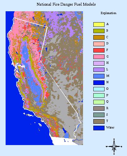
Figure 1. National Fire Danger Rating System fuel models.
The Mediterranean climate zone of California is of special importance to fire managers because of the large population adjacent to highly flammable wildlands. The Mediterranean chaparral vegetation types are fire-induced and have a high capability to withstand frequent burning. These vegetation types may have evolved features that make them more flammable: resinous oils, high surface-to-volume ratios, and a majority of stems less than 1 cm in diameter (Mutch 1970 and Biswell 1974),
Factors related to both climate and human activity help explain the high incidence of forest fires in the California Mediterranean region:
California has a distinct Mediterranean climate because of its winter concentration of rainfall and extreme summer drought (Ashmann 1973). The diverse topography of California represents all the variance allowable within the Mediterranean climatic type. Coastal areas have extremely cool summers and almost completely frost-free winters. A sheltered valley 20 miles inland can have extremely hot summers and brief winter frosts. The precipitation in California correlates positively with elevation and latitude of a Mediterranean climate (Ashmann 1973).
The NFDRS fuel model map (figure 1) was developed from a combination of vegetation types from the North American Land Characteristics data base (Loveland and others 1993), Omernik's (1987) ecoregion map, and field sampling of 2,560 plots. Each combination of vegetation type and ecosystem class was preliminarily identified to an NFDRS fuel model (table 1) ; this identification was based on assignment of the majority of plots in each combination of land cover and ecoregion. These preliminary fuel models were evaluated and corrected by knowledgeable U.S. Forest Service field personnel (Burgan and others In preparation). The NFDRS fuel model map provided information on the loadings of live and dead fuels (table 1) (Bradshaw and others 1983).
The RG was described by Burgan and Hartford (1993) as expressing how green each cell is relative to the range of greenness.
                                 (NDVI - NDVImin)
                         RG =  ------------------ * 100
                               (NDVImax - NDVImin)
Maximum and minimum NDVI values were calculated for the period 1989 through 1995. The RG provided an indication of the quantity of live vegetation and was used to calculate the proportion of the potential live fuel load.
The 10-h TLFM provided the moisture content of dead fuels - 1 inch in diameter. The 10-h TLFM can be calculated from temperature, relative humidity, and the state-of-the-weather (Fosberg and Deeming 1971). Additionally, fire weather stations measure 10-h TLFM daily at 1400 local time. The 10-h TLFM was considered the proper measurement for the Mediterranean ecosystem because of the majority of chaparral stems being less than 1 cm (Biswell 1974). The 10-h TLFM point observations were interpolated into a 1-km grid cell continuous surface using inverse distance weighting with an exponent of one.
The FPI model used the NFDRS fuel models as a basis for estimating live and dead vegetation loads as a function of RG, which changes every 7 or 14 days, depending on the compositing period, and daily variance of 10-h TLFM. The FPI model was calculated daily. Ten-h TLFM were used for the same days comprising an RG composite.
Geographic information system (GIS) processing used Environmental Systems Research Incorporated ArcInfo2 software, specifically the GRID module for cell-based processing and Arc Macro Language (AML) for programming.
Splus2 and SPSS2 were used to make statistical calculations. Stepwise multiple regression used an of 0.01 for adding variables and 0.02 for removing variables.
The geographic locations of 36,720 fires in California between 1990 and 1994 were collected from the data bases of the California Division of Forestry, U.S. Forest Service, U.S. Bureau of Land Management, and other Department of the Interior agencies. These data bases were combined into a common data structure and converted to a point coverage. The geographic locations of 722 fires were in error and were eliminated from the data base by clipping the historical fire point coverage to the California State boundary. This resulted in a point coverage of 35,998 fires. The annual distribution of fires was 7,610, 6,482, 8,547, 6,298, and 7,061 in 1990 through 1994, respectively.
Table 2 shows the distribution of fires by year and size class for those fires with area information. Most fires were in the 0 - 0.25-acre class. More fires were in the larger classes in 1994 than for the other years.
Data from 341 weather stations were obtained for 1990 through 1994. These weather stations recorded a total of 186,208 daily observations. Generally, between March and June, there were 50 weather stations reporting; between June and October there were 170 stations reporting. There were 183,521 10-hr TLFM measurements between 1990 and 1994. Some weather records did not have a corresponding location due to the elimination of a weather station from the data base. These missing locations accounted for approximately 30 weather observations in the early years and diminished to about five observations in 1994.
The RG was calculated for the years 1990 through 1994 (table 3). The 1990, 1991, and 1992 data sets were composited every 14 days, and the 1993 and 1994 data sets were composited every week.
The fuel model was implemented using ArcInfo GRID, using the following code fragment where %rg% is the variable for the RG grid, nfdrfuel.live is the amount of live vegetation in the National Fire Danger Rating System fuel model, nfdrfuel.dead is the amount of dead fuels in the National Fire Danger Rating System fuel model, and tmp10hr is the 10-h TLFM.
   docell

      rgfrac := rg/%rg% / 100.

      lfl := rgfrac * fm/nfdrfuel.live
      dfl := (1.0 - rgfrac) * fm/nfdrfuel.live + fm/nfdrfuel.dead

      lr := lfl / (fm/nfdrfuel.live + fm/nfdrfuel.dead)
      dr := dfl / (fm/nfdrfuel.live + fm/nfdrfuel.dead)

      tenfrac := tmp10hr / 30.0

      /* if tmp10hr > 30, fully saturated with moisture
      tenfrac := con(tenfrac > 1.0, 1.0, tenfrac)

      fpot := 100. - (rgfrac * lr + tenfrac * dr) * 100

      fpot := int(fpot)
      fpot := con(fpot > 100, 100, fpot)
      fpot := con(fm/nfdrfuel == 13, 101, fpot)       /* ag land
      fpot := con(rg/%rg% == 0, 0, fpot)                /* clouds
      fpot/fpot%day% = con(rg/%rg% == 255, 255, fpot)  /* water

   end
The RG, scaled between 0 and 1, was used to calculate the amount of live fuels (lfl) in an NFDRS fuel model. The amount of dead fuels (dfl) in the NFDRS fuel model were the dead fuels and the remainder of the live fuels that were not accounted for in lfl. FPI (fpot) equals lfl divided by the total amount of fuels weighted by RG plus dfl divided by the total amount of fuels weighted by the 10-h TLFM. FPI was scaled between 0 and 100. Cell values of 0, 101, and 255 were used to record clouds, agricultural land, and water, respectively.
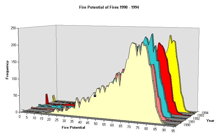
FPI grids were calculated for 239, 238, 195, 236, and 194 days in 1990 through 1994, respectively. The locations of fires were compared to these FPI grids to give the FPI of fires (figure 2), which were similar for all years. Few fires occurred at low FPI values, and the maximum number of fires occurred at an FPI in the low 70's. The number of fires decreased rapidly after an FPI of 80.
Fire density was determined for each FPI class, to determine the relationship between FPI and fire frequency. Fire density was calculated by dividing the number of fires in an FPI class by the total number of cells in that FPI class. Fire density was used to help remove the high correlation with area in both distributions of fire cells with FPI and the landscape cells with FPI. There was a strong positive relationship between FPI class and fire density (figure 4). Linear regression showed statistically significant relationships between FPI classes and fire density yearly and with all years combined (table 4). FPI was limited to the range between 15 and 80 because there were few fires below 15 and above 80. Management restrictions of forest access and increased public awareness of fire danger were in place to limit the potential for human-caused fires at FPI of 80 and above.
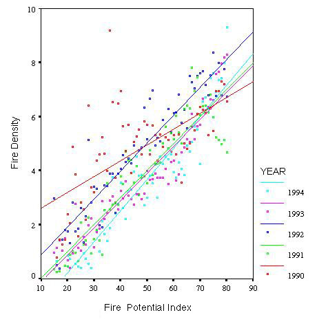
Multiple regression, with year indicator and interaction terms using 1994 as the base year, indicated that the linear equations for FPI class and fire density were statistically identical for 1991, 1993, and 1994 (r2 = 0.825, df = 1 and 318, F = 375.05, p < 0.000). The equation of this line was:
Fire Density = 0.104 FPI - 1.322
The linear equation for 1990 was different from these years in both slope and intersect. The linear equation for 1992 had a greater intersect than the other years but the same slope. That is, for a given FPI class in 1992, fire density was higher than in the years 1991, 1993, and 1994.
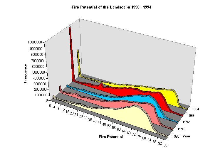
The results are encouraging because the FPI model appears to have predicted the fire situation. There was little annual variation in the frequency distributions of the FPI of fires (figure 2). However, there were annual variations in the frequency distributions of the FPI of the landscape (figure 3). The increase in larger fires in 1994 (table 2) may be reflected in the frequency distribution of FPI of the landscape being skewed to higher FPI.
The power of the FPI was illustrated by the single regression line describing 1991, 1993, and 1994 fire density. Further work is required to explain why the relationship was weaker in 1990 than in the other years and why the slope was greater in 1992 than in the other years. Possible reasons could be problems with the NDVI data, changes in the calibration in the AVHRR sensor, accuracy in the location of fires, the 1-km resolution of the analysis, or the inclusion of Nevada in the landscape. In any case, 72 percent of the variation in fire density was explained by FPI when all years were combined (table 4).
There were problems in locating historical fires by latitude-longitude coordinates. Seven hundred twenty-two fires were deleted from the data base because they occurred outside California. Determining latitude-longitude is difficult; it is hoped that increased use of GPS can minimize these errors in the future.
The geographic locations of the weather stations were more accurate than the locations of the historical fires; however, there were some California weather stations occurring outside of California when plotted. A more serious problem was the lack of geographic locations for some stations once reporting was discontinued. A data base needs to be maintained that holds information on all historic and current weather stations so that the complete data base of weather observations can be used.
The main improvement required for the FPI model is the interpolation of the point weather observations to a continuous surface. These results were calculated using a simple inverse distance weighting interpolation. This method did not take into account topographic and orographic variation, distance from the ocean, and distance from mountainous barriers. Further work should develop a better method to interpolate meteorological data between weather stations.
If this model were to be used in an operational setting, the use of weather observations and RG would need to be modified. This model used the weather observations for the same days that the NDVI was composited. In an operational use of the model, this cannot be done or the calculations of FPI would be delayed. Operational use of the model requires that the RG would be for one period of time and weather observations would follow the compositing date. This modification should not affect the results significantly. The NDVI changes slowly with time; consequently the RG should not be greatly affected.
Other factors could be added to the model to simulate human causes of fire, like proximity to roads, power lines, and houses, as was done by Chuvieco and Congalton (1989), Chou and others (1990 and 1993), and Chuvieco and Salas (1996). These would be useful factors to include, but are more suited for smaller study areas where detailed GIS data layers are available.
The use of GRID was a benefit to these calculations. GRID uses a data base with images for its calculations to reduce the number of data layers. In this case, one grid of NFDRS fuel models was used rather than separate grids of live and dead fuel loadings. This not only saved disk space but also reduced the number of grids to maintain and process.
More importantly, intermediate operations are made in memory using the GRID DOCELL command rather than written out as separate grids. This again reduces the number of grids to track and disk space required. In this model the DOCELL command created one grid rather than the 13 that would have been created otherwise from the FPI model.
The FPI model complements the NFDRS in that they use the same fuel models. The FPI model calculates fire danger values for the total geographic extent of the study area by its use of NDVI, fuel model maps, and weather stations. The NFDRS calculates fire danger for specific point locations only.
The results of the FPI in the California Mediterranean ecosystem indicate that it is potentially a valuable fire management tool for land management agencies. It is hoped that the FPI will be equally useful in the Mediterranean ecosystems of Chile, Mexico, and Spain. The FPI methodology could be used for future comparisons of how the Mediterranean ecosystems respond at different geographic locations throughout the world.
1. Hughes STX Corporation. Work performed under U.S. Geological Survey contracts
1434-92-C-4004 and 1434-CR-97-CN-40274.
2. Any use of trade, product, or firm names is for descriptive purposes only and does not imply
endorsement by the U.S. Government.
Dave Sapsis, California Division of Forestry, supplied the weather data and locations of fires on
California Division of Forestry and Bureau of Land Management lands. Paul Olsen prepared
movie loops of the daily FPI images. Bruce Wylie provided many helpful suggestions
throughout the project. Stephen Howard and Eric Wood provided useful comments on earlier
drafts of this paper.
Ashmann, H.A. 1973. Distribution and peculiarity of Mediterranean Ecosystems. Pages 11-19.
In: F. Di Castri and H. A. Mooney (Eds.), Ecological Studies, Analysis and Synthesis, Vol. 7.
Springer-Verlag, Berlin. 405 pages.
Bailey, Robert G. 1996. Ecosystem Geography. Springer. New York. 204 pages.
Biswell, Harold H. 1974. Effects of fire on chaparral. Pages 321 - 364 In T.T. Kozlowski and
C.E. Ahlgren (Eds.) Fire and ecosystems. Academic Press, New York. 542 pages.
Bradshaw, Larry S., John E. Deeming, Robert E. Burgan, and Jack D. Cohen. 1983. The national
fire-danger rating system: technical documentation. Gen. Tech. Rep. INT-169. Ogden, UT: US
Department of Agriculture, Forest Service.
Burgan, Robert E., Robert W. Klaver, and Jacqueline M. Klaver. In Preparation. Mapping fuel
models and fire potential with satellite and
surface observations.
Burgan, Robert E. and Roberta A. Hartford. 1993. Monitoring vegetation greenness with satellite
data. Gen. Tech. Rep. INT-297. Ogden, UT: US Department of Agriculture, Forest Service.
Chou, Yue-Hong, Richard A. Minnich, and Richard A. Chase. 1993. Mapping probability of
fire occurrence in the San Jacinto Mountains, California, USA. Environmental Management
17(1):129-140.
Chou, Yue-Hong, Richard A. Minnich, Lucy A. Salazar, Jeanne D. Power, and Raymond J.
Dezzani. 1990. Spatial autocorrelation of wildfire distribution in the Idyllwild Quadrangle, San
Jacinto Mountain, California. Photogrammetric Engineering and Remote Sensing
56(11):1507-1513.
Chuvieco, Emilio and Russell G. Congalton. 1989. Application of remote sensing and
geographic information systems to forest fire hazard mapping. Remote Sensing of the
Enviuronment 29:147-159.
Chuvieco, Emilio and Javier Salas. 1996. Mapping the spatial distribution of forest fire danger
using GIS. International Journal of Geographical Information Systems 10(3):333-345.
Deeming, John E., Robert E. Burgan, and Jack D. Cohen. 1977. The national fire-danger rating
system - 1978. Gen. Tech. Rep. INT-39. Ogden, UT: US Department of Agriculture, Forest
Service.
Fosberg, Michael A., John E. Deeming. 1971. Derivation of the 1- and 10-hour timelag fuel
moisture calculations for fire-danger rating. Research Note RM-207. Fort Colins, CO: US
Department of Agriculture, Forest Service.
Loveland, T.R., D.O. Ohlen, J.F. Brown, B.C. Reed, and J.W. Merchant. 1993. Protype 1990
conterminous United States land cover characteristics data set CD-ROM. EROS Data Center.
U.S. Geological Survey CD-ROM 9307, 1 disc.
Minnich, Richard A. 1988. The Biogeography of Fire in the San Bernardino Mountains of
California, A Historical Study. University of California Publications in
Geography, Volume 28. University of California Press, Berkeley. 121 pages.
Mutch, R.W. 1970. Wildland fires and ecosystems - a hypothesis. Ecology 51:1046-1051.
Omernik, James M. 1987. Ecoregions of the conterminous United States. Annals of the
Association of American Geographers 77(1): 118-125.
Jacqueline M. Klaver1ACKNOWLEDGMENTS
REFERENCES
TABLES
(Deeming and others 1977 and
Bradshaw and others 1983).
Fuel Model
Description
Live Fuels (Tons/Ac)
Dead Fuels (Tons/Ac)
A
Western grasslands vegetated by annual grasses and
forbs. Brush and trees occupying less than one-third of
the area. Quantity and continuity of the ground fuels
vary greatly with rainfall from year to year. Examples
are cheatgrass and medusahead types. Some pinyon-juniper, sagebrush-grass, and desert shrub
stands.
0.3
0.2
B
Mature, dense fields of brush 6 ft. or more in height.
One-fourth of aerial fuel is dead. Example is the
California mixed chaparral 30 years or older.
11.5
8.0
C
Open pine stands. Perennial grasses and forbs are
primary ground fuels, but there is significant needle
litter and branchwood. Examples are longleaf, slash,
ponderosa, Jeffery, and sugar pine. Some pinyon-juniper stands.
1.3
1.4
D
Palmetto-gallberry understory pine overstory.
3.75
3.0
F
Mature closed chamise stands and oakbrush fields.
Also young, closed stands and mature, open stands of
California mixed chaparral. Some open stands of
pinyon-juniper.
9.0
6.0
G
Dense conifer stands with heavy accumulation of litter
and downed woody material. Examples are hemlock-Sitka spruce, Coast Douglas-fir, and
windthrown or
bug-killed stands of lodgepole pine and spruce.
1.0
21.5
H
Stands of short-needled conifers (white pines, spruces, larches, and firs). Healthy stand
with sparse undergrowth and a thin layer of ground fuels.
1.0
6.5
L
Western perennial grasslands.
0.5
0.25
M
Agricultural Lands
0.0
0.0
N
Very coarse grass such as the sawgrass prairies of south
Florida. Marsh situations where the fuel is coarse and
reedlike. One-third of the aerial portion of the plants is
dead. Fast-spreading, intense fires can occur even over
standing water.
2.0
3.0
O
Dense, brushlike fuels of the Southeast United States. The plants are typically over 6 feet
tall and are often found under an open stand of pine.
7.0
10.0
P
Closed stands of long-needled southern pines. A 2- to 4- inch layer of lightly compacted
needle litter is the primary fuel.
1.0
2.5
Q
Upland Alaskan black spruce or jack pine stands of the
Lake States. The stands are dense but have frequent
openings filled with usually inflammable shrub species.
The forest floor is a deep layer of moss and lichens, but
there is some needle litter and small-diameter
branchwood.
4.5
7.5
R
Hardwood areas after the canopies leaf out. Used
during the summer in all hardwood and mixed conifer-hardwood stands where more
than half of the overstory is deciduous.
1.0
1.5
S
Alaskan or alpine tundra on relatively well-drained sites. Grass and low shrubs are often
present, but the principal fuel is a deep layer of lichens and moss.
1.0
2.0
T
Sagebrush-grass type of the U.S. Great Basin and the Intermountain West and scrub oak
and desert shrub types. The shrubs burn easily and are not dense enough to shade out grass and
other herbaceous plants. The shrubs may occupy at least one-third of the site.
3.0
1.5
Year
1990
1991
1992
1993
1994
Fire Size
(Acres) 0 - 0.25
2,595
2,174
2,738
1,465
1,780
0.25 - 10
748
537
741
520
716
10 - 100
97
61
115
139
140
100 - 300
28
23
40
44
38
300 - 1,000
22
6
34
33
43
1,000 - 5,000
17
6
23
17
36
> 5,000
12
1
11
12
17
Total
3,519
2,808
3,702
2,230
2,770
1. Except first and second grids, which were 14-day composites.
Year
Begin Date
End Date
Interval
Number of Grids
1990
15 March
25 October
14-days
17
1991
14 March
24 October
14-days
17
1992
19 March
29 October
14-days
17
1993
18 March
28 October
7-days
33
1994
17 March
15 September
7-days1
26
Year
r2
F
df
p
1990
0.44
49.96
1 and 63
0.000
1991
0.85
352.24
1 and 64
0.000
1992
0.87
443.31
1 and 64
0.000
1993
0.90
585.50
1 and 64
0.000
1994
0.88
444.72
1 and 58
0.000
1990 - 1994
0.72
840.13
1 and 321
0.000
Senior Scientist
Telephone: (605) 594-6961
Fax: (605) 594-6568
jklaver@edcmail.cr.usgs.gov
Robert W. Klaver1
Senior Scientist
Telephone: (605) 594-6067
Fax: (605) 594-6568
bklaver@edcmail.cr.usgs.gov
Science and Applications Branch
USGS EROS Data Center
Sioux Falls, SD 57198
Robert E. Burgan
Research Forester
Telephone: (406) 329-4864
Fax: (406) 329-4825
rburgan/int_missoula@fs.fed.us
Intermountain Fire Sciences Laboratory
P.O. Box 8089
U.S. Forest Service
Missoula, MT 59807