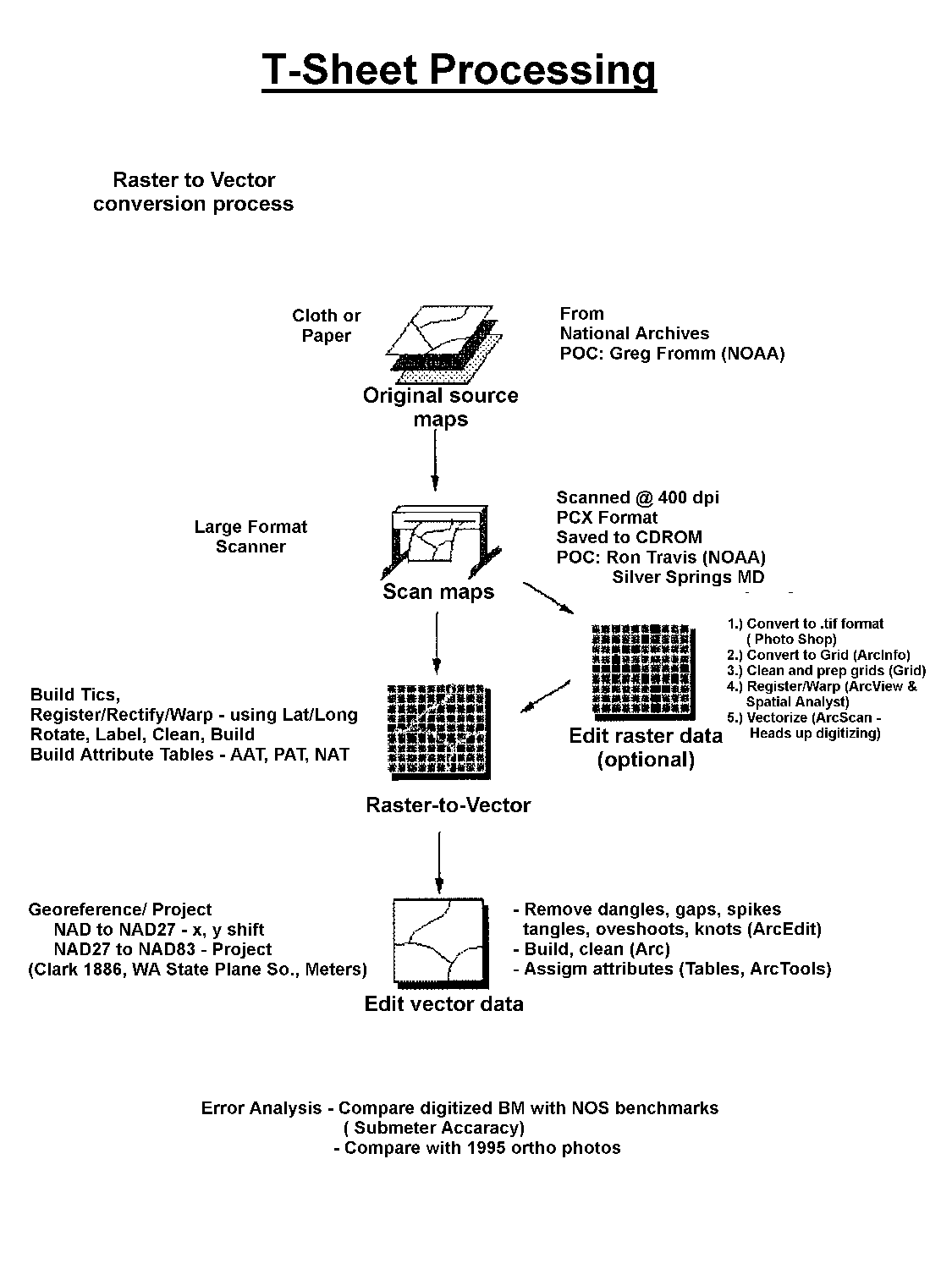
Map Vectorization Process
Robert H. Huxford
The Washington State Department of Ecology and the National Ocean and Atmospheric Agency (NOAA) have joined forces, in a Coastal Mapping Partnership, to develop advanced methods to vectorize shorelines. The source for historical shorelines come from rasterized historic and contemporary National Ocean Survey (NOS) topographic survey sheets. The methods developed, integrate ArcInfo, ArcScan, Grid, ArcTools, Arcview, and Spatial Analyst. The system blends customized ArcView scripts with ArcInfo AML’s into a seamless integrated process that greatly simplifies and speeds up the vectorization. Most T-Sheets now reside in the National Archives. Shorelines as for back as 1850 have been recovered and now can be compared with present data to identify changes in the Washington coast.
The National Oceanic and Atmospheric Administration (NOAA) has undertaken a data rescue project to convert historical and contemporary topographic sheets (T-sheets) from paper to a digital format. These T-sheets are detailed survey maps that were produced to provide coastlines for use on navigation charts issued by the National Ocean Service (formerly the U.S. Coast and Geodetic Survey). The information content of T-Sheets varies. At a minimum, each T-sheet contains the mean high water line as derived from field survey; survey marker locations used to provide control for the field work; a coordinate system formed by longitude and latitude lines; and graphic representation of the vegetation inland from the coast. Most of the T-Sheets done for the state of Washington are at a scale of 1:10,000 or 1:20,000. In addition, many maps include topography and additional longitude and latitude lines that represent translations between old and new datums or projections.
This report will discuss and explain methodologies and tools used in the Coastal Mapping Partnership with NOAA to vectorize the historical shoreline. The tools and methodologies were developed by NOAA’s Coastal Services Center (CSC) in Charleston, South Carolina. The scope of the project is to develop methods to vectorized shoreline from raster images of historic and contemporary NOS topographic survey sheets. The project was set up as a multi-year endeavor with funding renewed on an annual basis. NOS provided raster images, technical assistance, training, macros, and consultation necessary to complete this task. The State of Washington provided the computing equipment, staff and administrative support necessary to insure the completion of the project. At the conclusion of the project, the State of Washington is to provide NOS with a Washington vector shorelines on a suitable GIS medium (i.e.: ArcInfo coverages).
In this data rescue project, the original paper and cloth maps were scanned at 400 dots per inch using a large format scanner at NOAA. The scanned data was then saved to CDROM disk for archive. This scanning process has been successful in saving these important informational resources from loss, and has now made them available outside the National Archives. The scanned images, however, have no attribute information – they are just images of a map. To extract and assign attribute information from the scanned image, it is necessary to convert the information on the raster image to vector lines (arcs) that can be described by X, Y coordinate pairs.
The Players:
The Plan: To develop an automated process for turning scanned raster-based NOAA topographic survey (T-sheets) for the northwest coast into a complete region-wide vector database. This effort will be accomplished by use of a Geographic Information System (GIS), ArcInfo.
The Purpose: Benefactors from the completed work will be Coastal Resource Managers participating in an ocean planning GIS for the northwest. Shoreline data is a critical framework element for any ocean related GIS activity. Oil spill mitigation, shore erosion and deposition studies, and endangered species protection are just a few examples of a need for an accurate shoreline data layer.
Hardware:
Software:
Data:
Map Vectorization Process
Conversion Process Accuracy’s
Although the accuracy of NOAA topographic sheets has been shown be very good (Byrnes et al. 1991, Anders and Byrnes 1991), there are few methods defined to determine the statistical accuracy of the data conversion process. Because future research in Washington involved quantitative analysis of changes in configuration of the Washington shoreline and its change in position over time, it was essential that we be able to quantify the accuracy of this data conversion process.
Our goal was to induce the minimal amount of error possible in the scanning or vectorization process and to correct for any shrinking or warping that might have occurred in the original maps. By comparison, U.S. Geological Survey 1:24000 topographic maps are only accurate to approximately 40 feet, or about 12.2 meters, for a well defined point. It was our hope that the T-sheet conversion process would produce accuracy’s one half of that value. The additional accuracy is needed for a concurrent erosion project being run by the USGS and Washington’s Department of Ecology. In this project we need to be able to measure erosion or accretion quantitatively, hence the need for a much higher level of accuracy.
Methodology for Extraction Vectors from Raster Images
The process of converting the raster data to vectors is a five-step process. First, the projection and datum used on the source map are identified [i.e., local datums, North American Datum (NAD), North American Datum of 1927 (NAD27), or North American Datum of 1983 (NAD83)]. Second, the raster image are registered to the longitude and latitude lines on the original map. Third, the images are transformed into degrees and decimal degrees. Fourth, the coastline data on the raster images are vectorized and attributes are added to obtain the final line work that is saved in a digital format. Finally, these vectorized shorelines are projected into a common datum, in our case (NAD83).
Several sources may introduce error in the final digital data. The primary sources are map shrinkage, locational accuracy of the longitude and latitude lines, scanner errors, datum accuracy, datum transformation errors, and digitizing errors.
The methodology currently being used by the NOAA data rescue project is to register the scanned map images using the longitude and latitude lines that were drawn on the source maps by the original cartographer and survey teams. These original datums are finally converted to the most currently used datum, NAD83 using available transformation algorithms. These original datums were in local datums, the North American Datum (NAD) (historical maps older than the 1927) or the North American Datum 1927 (NAD27) (contemporary maps). The survey teams also plotted the location of the benchmarks or survey marks used during their fieldwork. Some maps contained more than one datum graticule on the sheet. For the NOAA data rescue project, all maps were converted to the newest datum NAD83 so maps from different dates could be compared with each other. The NGS benchmarks/survey marks on these maps were compared with current NGS benchmark data sheets to assess the overall accuracy of the process.
The Washington Program:
Startup - The project was set up to be a multi-year endeavor where funding would be renewed on an annual basisThe major thrust of the first year was to create the infrastructure necessary to complete the work. The Washington portion of this NOS study started the last week in October 1996. This was the first year of a three year project to develop shoreline data for the state. The scopes of work and budgets for following years are to be negotiated at the beginning of each year and are subject to availability of funds and the mutual agreement of both parties. I effectively started on the November 1, 1996.
Initial Steps - After the project started, it was determined ArcInfo and ArcScan from the Environmental Systems Research Institute (Esri) company was to be used as the primary software to process the scanned topographic sheets. The Department of Ecology already had ArcInfo, but it was necessary to acquire an ArcScan license to be able to process the scanned images. ArcScan software was installed in December 1996 so local in-house training and familiarization could be accomplished. Later, a formal, one day ArcScan training class was attended in Redlands California at Esri in January 1997. Just recently, new pieces in the software suite, ArcView and Spatial Analyst, have been added to improve the integrated package. With these new pieces are Avenue scripts and ArcInfo AML’s written at NOAA’s Coastal Services Center by Jeff Cowen, The new scripts and AML’s greatly simplify and speed up the process.
Methodologies - During the months of January, February, and March 1997, local procedures and methodologies were developed to facilitate the production of the vector maps. The methods and procedures have been written out to serve to document how the vector maps were produced. This development process is ongoing as new methods are developed or old ones are improved. Some of the local procedures include:
Local Washington Data Catalog - In late December 1996, map information catalogs were received from NOAA depicting topographic and hydrographic sheets available for Washington and surrounding areas. An initial review of the catalogs showed that there were 1284 sheets listed on 63 separate map indexes. However over a third of the T-Sheets listed were on one or more index maps, making it difficult to determine if a particular T-Sheet was unique. Because of this, a relational database was created that showed all index maps that a particular T-Sheet appears on. The database was expanded to include:
The layout of this database allows the search or sorting of T-Sheets by any of the above fields. Once the database was complete, status pages were generated for each map index showing the status of all T-Sheets on that index page. These status pages were then combined with their associated index maps to produce a catalog that shows the complete status of all T-Sheets. From the database, I was able to determine that there were 951 unique topographic or hydrographic maps for Washington. Approximately a third of the maps are shown on two or more indexes. Of those 951 maps, We now have 166 scanned maps from NOS.
Data Arrival - The first raster images of T-Sheets from NOS arrived in the first week in December 1997. The two CD-ROM’s contained approximately 150 contemporary maps from 24 map indexes. A third CD arrived the second week in February containing historical T-Sheets needed for a coastal erosion project at Ecology. Because of the critical nature of historical T-Sheets information, I was allowed by NOAA to give these historical shorelines priority in processing.
New Methods form CSC - On May 1997, a T-Sheet vectorization workshop was conducted by the Coastal Services Center in Charleston, South Carolina. The purpose was to bring participants on the west coast up to speed on new methods the CSC was using for the digitizing their T-Sheets. The most significant updates were the integration of ArcView and ArcView Spatial Analyst into the process. All the processes were simplified and greatly automated. The time now required to process T-Sheet has been significantly reduced. The AML’s and scripts needed to implement the system developed by CSC for Washington have been down loaded and installed on our system. The final missing piece, ArcView Spatial Analyst. was added in late 1997 to complete the software suite needed for map production.
Converting the Data to grids
The first step in converting our map images to vector map is to get the image files into a format that ArcInfo can process. The images were scanned by NOAA and came to us as very large compressed .pcx files. These files are first viewed in Adobe Photoshop, the only program we could find that would effectively read these large compressed files, and then converted into a format that ArcInfo could readily use. In Photoshop, the images were uncompressed, cleaned and trimmed. They are then saved as uncompressed .tif files, cataloged, and archived to a CDROM for later use. When I am ready to process the image, I transfer it to its own folder in my working directory. This folder will contain all the files associated with this particular T-Sheet. After the image file is in its own folder, we make this folder our working directory. At the Arc prompt we type in the following command...
Arc: imagegrid t_sheet.tif t_sheetgrdWhere "t_sheet.tif" and "t_sheetgrd" are the name given these files.
This converts the raster file into an ArcInfo Grid and may take several minutes to finish depending on the speed of the computer. Once finished, we are ready to register the grid using our new ArcView extension created at CSC. Quit out of Arc and go into ArcView.
Arc: quit
unixprompt: arcview
Registering grids using ArcView
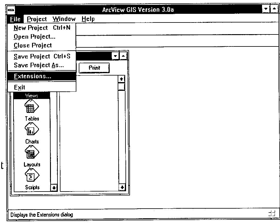
Once the ArcView project window appears, we click on the "File" pull-down menu and select the option "Extensions..." This will open a new window showing the available extensions to load into the view. We first select "Spatial Analyst" extension by checking the box on the left of the option and Click OK. We again, pull down the "Extensions..." option and select the extension called "Register T-Sheets", then click OK.
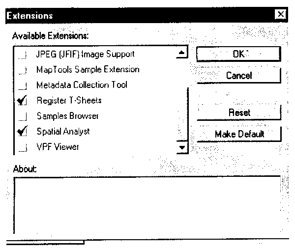
Getting Extensions
Extension Menu
Loading the Extensions
This loads the programs that perform the registration process. We pull down the "Extensions..." option one last time, and select the extension called "CellTool Extension". This adds a number of helpful tools to our View's GUI.
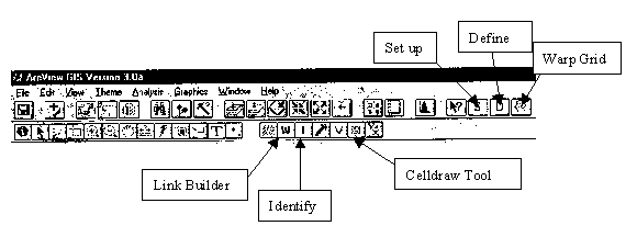
Extension GUI
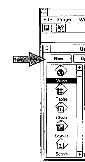
New View Button
We open up a view by clicking on the "New" button on the project window while the View document is active. Our View window will open, and its GUI will look like this with the added buttons and tools on the right hand side of the bar. We will discuss what each one does as we continue.
Displaying the Grid
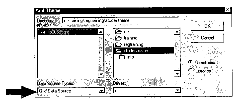
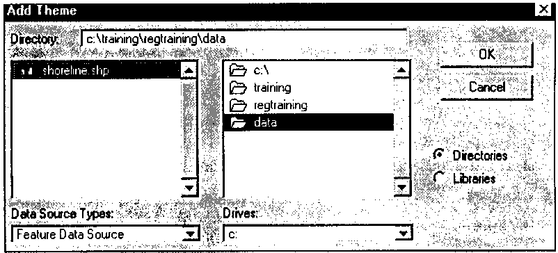
Add Theme Button
Using the Add Theme button, we change the Data Source Type option on the bottom of the "Add Theme" pop-up window to be "Grid Data Source". We want to be sure to add in the grid we created as a Grid and not as an Image! The registration program will not accept images.
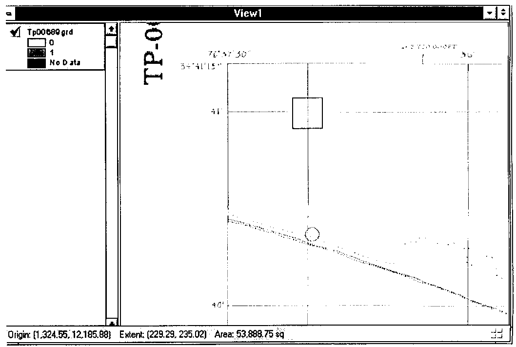
Once the grid is added to the view, we turn it on by checking the theme's box. The colors are randomly assigned and may make viewing the grid difficult. We generally use the Legend Editor to change the colors so that viewing is-made easier. A good rule of thumb is to change the background and the "No Data" color to be transparent. The "0" and "1" colors can be any contrasting color. I prefer darker lines on a lighter background.
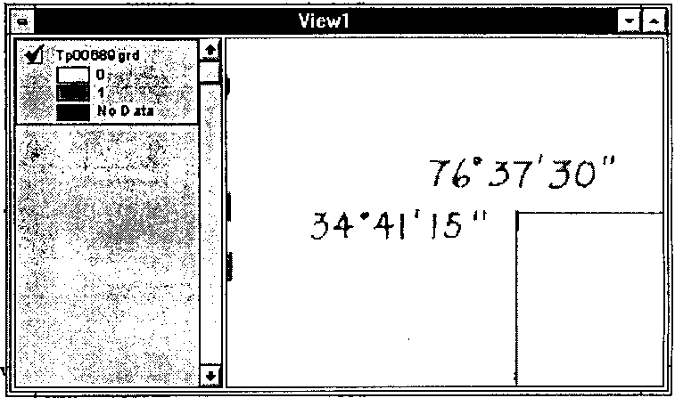
T-Sheet Corner
Working Directory
Beginning the Registration
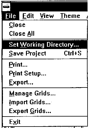
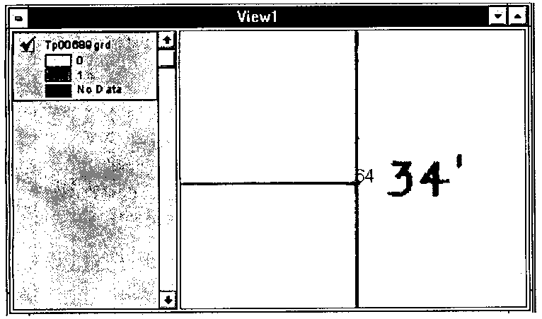
Using the Zoom-In tool, we window in on the upper-left corner of the grid and find the latitude and longitude coordinate pair. Notice the example above shows the numbers clearly displayed. We now want to direct ArcView to the directory that our files will be written in. This should be the folder that was created in our home directory when we imported the T-Sheet image file. I find it best to keep all the files, ArcView and ArcInfo, in the same location while I am processing a particular T-Sheet. We pull down the "File" menu and select "Set Working Directory… ".
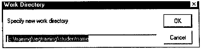 Set Working Directory
We change our directory pathway to the folder we put your image file in, instead of what is shown here and Click OK. We are now ready to input the upper-left and lower-right coordinate pairs of this grid.
Whole Rectangles
But before we do, notice that the upper-left (and lower-right) corners are partial rectangles? This ArcView registration script procedure will only work on the corners of whole rectangles. This has to do with the count of rows and columns used In the script to display the tic numbers, and if a row or column are partial, then it throws off the graphics display and the script will not work correctly. Therefore, one needs to zoom out to an area like the one shown above, and then zoom in to a whole gridline intersection like the one that is shown in the box above.
Setting up the Tics
We click on the "Set Up" button [S] and select the grid you want to warp. This will give a listing of all the grids in our View's table of contents. Click OK.
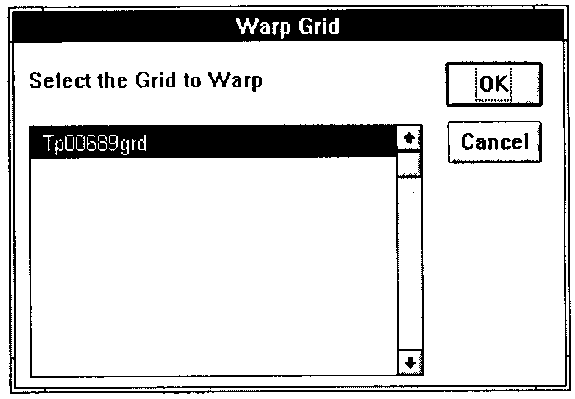
Select a Grid
Input Data
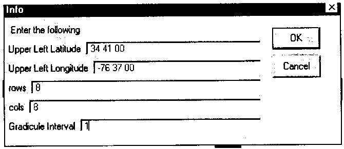
At this point we want to write down the upper-left latitude/longitude coordinate pair which defines the beginning of a grid square, the number of rows, number of columns, the graticule interval, and the scale of the T-sheet. It takes a moment panning around the grid to collect this information and we record it on a sheet of paper. We will need to report most of it in the next step.
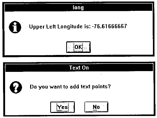
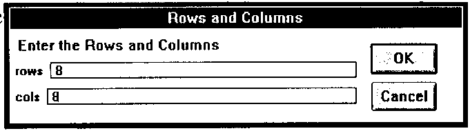
We are now ready to click on the "Define" button [D]. We now have to input the latitude and longitude for the gridline we are zoomed in on. Be sure to include a negative value for the longitude. Next, we input the number of rows and columns of whole rectangles. There is one row and column for each longitude and latitude line. This is just to get the graphic tic-ids to line up in place. Next, we need to define the graticule interval. Because this map is in one-minute intervals, we will define it as "1". If the grid lines were 30 seconds apart then the graticule interval would be .5 Click OK.
A series of message boxes will then appear informing us of several things. First, the program recognizes the distance in decimal-degrees of the graticule interval. The next two are echoing the latitude and longitude location of the first tic in decimal-degrees. Then, the user is prompted to add the text points as a file in the Tables Document. Always choose "Yes" because the following program will read this file if it exists, The resulting table is displayed below as it should look to the user.
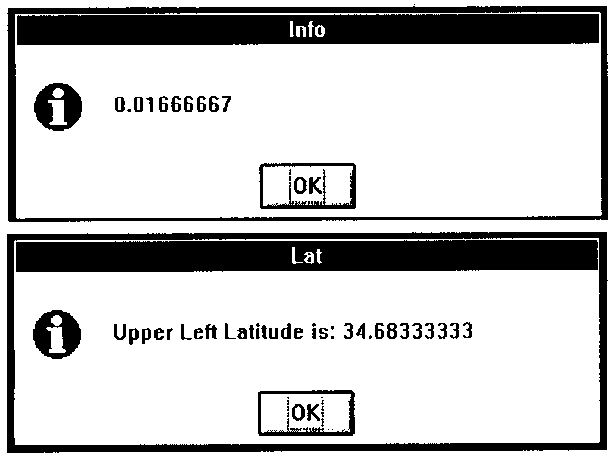
Graticule/Lat
Long/Text
Drawing the Tic-Ids
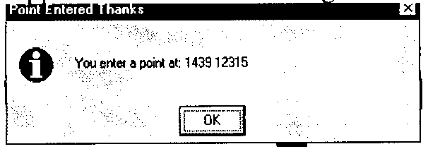
We are now ready to have the tic-ids draw to the screen. We click on the "Identify" button. [ I ] The following message box will appear and we will want to add the upper-left tic location that we are zoomed in on. When we click OK the cursor will turn into a crosshair. Once we locate the approximate center of the gridline intersection and click the mouse, another window appears that tells us the coordinate location in "pixel space" of that selected location.

Upper Left Corner
Points Entered
Text File
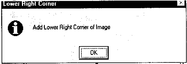
Lower Right Corner
Points Entered
we now use the "Zoom to Selected Theme" button to see the entire theme. We then use the "Zoom In" tool to find the lower-right corner. Once we are positioned on the intersection of the gridline, we click the "Identify" button again and click on the intersection. Again another window appears that tells us the coordinate location in "pixel space" of that selected location.
Rows & Columns
Drawing the Tic Ids (Part 2)
A pop-up window will again prompt us for the number of rows and columns. This is done so that the program will know what the intervals are that the graphic text will be displayed. We type in the same values as before and click OK.
Drawn Tics
Now the tic ids for every grid intersection are added to the view as a graphics file. We can now display them all by clicking on the "Zoom to Selected Theme" button again.
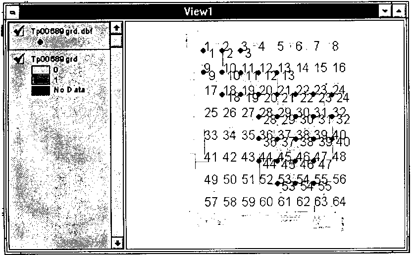
We will now begin the process of zooming in to certain tic id locations to capture the center pixel of the gridline intersection. Not all of the tic ids will be used in building the link file. Because additional error can be introduced in collecting tic ids that fall outside of the area that shoreline is located, we want to be selective.
Selecting the Right Tic Ids
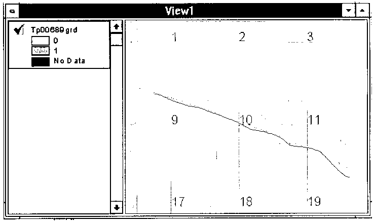
In the example below of the tic ids at the upper left of the grid, we can see how the shoreline runs through the rectangles of the gridline intersections. We would want to capture all of the pixels located under each of these tic ids with the exception of number 17. Every other tic id has some shoreline running through its rectangle. Therefore, we will focus on how to capture only those pixels on the corner of rectangles with shoreline data contain within.
Tic Ids
Zoomed In
We can begin anywhere on the grid, I prefer to go in an ascending order to capture the pixels. We zoom in to the intersection of tic id "1". One of the benefits of using this method of registration is that we can zoom right in onto the exact center pixel of an intersection. This is very difficult to do using ArcInfo's "register" program.
Heads-up Digitizing:
Perhaps the greatest advantage of using this integrated system is the ability to use heads-up digitizing. This method allowed us obtain accuracy not possible with a conventional digitizing board. With conventional methods it is only possible to digitize to about .5 mm consistently. This equates to approximately 5.0 meters on a 1:10,000 T-Sheet and double that for a 1:20,000 sheet. In contrast when a 1:10,000 T-Sheet is scanned at 400 dpi the width of each pixel is 0.0635 mm and equivalent to 0.64 meters on the ground. When the scanned image is oriented, registered, and rectified it was possible to do so to within two pixels or 1.2 meters. The auto tracing function in ArcScan also allowed us to digitize to the weighted center of a line. This is not possible using manual digitizing techniques. The accuracy of the original T-Sheets is therefore maintained in the transfer to digital form.
![]() Cell Draw Button
Cell Draw Button
Building the Link File
Once we have zoomed in close enough, we can determine which pixel is at the center of the gridline intersection by using the celldraw tool. When we click on the tool, a message box appears asking if we want to save the graphics that
Save Graphics?
it draws to the screen. I usually say "Yes" so that I can keep track of the intersections that I have processed. Move the cursor to what appears to be the center of the intersection. When we click on that position, a three-by-three grid cell is drawn which shows the location of the individual pixels.
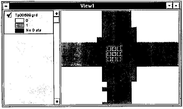
Pick Cell
Now it is possible to see the precise pixel that falls exactly in the center of the intersecting lines. Once we have determined which pixel we want to select, we click on the "Link Builder" tool. [W] The cursor becomes a bulls eye. We click on the pixel and see a pop-up box appear that prompts us for this tic id value. We type in its number and click OK.
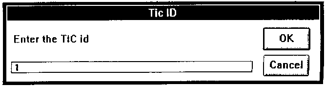
Tic ID?

Add Another
Building the Link File (Part 2)
Another window pops up to ask us if we would like to enter another point. We want to add in all of the points possible. It is necessary to have a minimum of 6 points to perform the second order bilinear transformation of the grid, so we click "Yes".
We need to zoom back out to find the next tic id. One helpful method is to use the "Zoom to Previous Extent" button. Continue zooming in, capturing the tic ids until you have collected all of the tic ids needed.
Once we have collected the last point, we answer "No" to the Collect More window. We are now ready to warp the grid!
Checking Our Work
It's important to have some "checks" built into the process of registration. After the link file is built, we want to add it into our Table document. We make the Table icon active on the Project window and click on the "Add" button. We change the "List Files of Type" drop-down list to "dBASE (*.dbf)", select the .dbf file in our directory, and click OK.
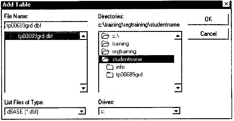
Add Table
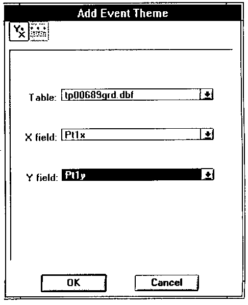
Add Event
We now want to add this file as an event theme into our view. We make the view window active and pull down the view menu and select "Add Event Theme". A pop-up window appears for us to enter the name of the .dbf file and the x, y fields. Enter the Ptlx and Ptly which indicates the pixel rather than the true decimal degree equivalents and click OK.
This .dbf file is now added to your view's table of contents as a theme and it can be turned on to see the location of the points.
Checking Our Work (Part 2)
The next step is to see if the entry of our tic ids were accurate. It is also nice to have the actual values draw along side the graphic text. We do this by first making the event theme active. We then pull down the Theme menu and select "Auto Label". A pop-up window will appear for us to specify the item in the .dbf file that we want to have labeled onto the screen. We select "Ticid" and select "Theme's Text Label Placement Property", then click OK.
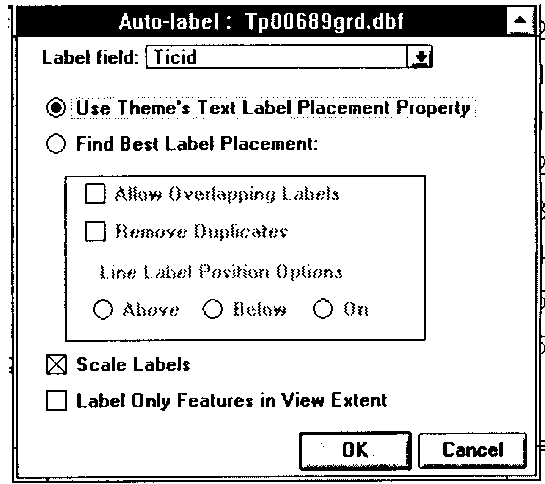
Auto Label
This will now draw the entered tic id values along side of the generated tic values. we look each one over to be sure that one was not incorrectly entered. Hopefully, our view will look something like the figure below. If so, we go ahead and proceed to the next step - warping of the grid.
If we need to remove a point, we can edit directly to the .dbf file and reenter new tic ids as before.
Ready to Warp
Warping the Grid To warp the grid, select the "Bex" button.
When we click on this button we will be asked to enter the scale of our grid. This is necessary because, an evaluation of the link file is made through an ArcInfo program called "LLSFit" which simply creates a file that shows the amount of RMS error in the link table. The amount of acceptable error is dependent on the scale of the grid. The smaller the scale (1:20,000) the fewer the number of pixels which can be in error (4 pixels). This conforms to National Map Accuracy Standards.
 Bex Button
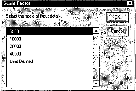 Scale Factor
Another benefit to performing the registration through this method is that a watch file is created that details exactly how LLSFit evaluated the link file. This is used for metadata purposes down the road if anyone has questions about which individual tic id was used in the grid warp. This is something else that ArcInfo's "Registration" command will not produce. we click OK after entering the scale factor.
Warping the Grid (Part 2)
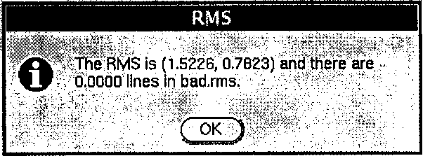
A system execute command is sent to run ArcInfo and perform the LLSFit command.
Once completed, a pop-up window will appear telling you the total RMS for the link file and how many records were "bad" or over the scale factor. If we have links that are bad and would like the program to continue, it will prompt us to delete the one that has the highest RMS and then will rerun the LLSFit again. It will continue to report back to us the RMS value and the bad link status until all of the links are within the accepted amount.
RMS Values
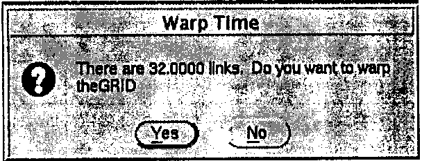
Warp the Grid
Once done, we will be told how many links are valid and asked if we would like the grid to be warped. If you answer "No" the program will terminate immediately. If we answer "Yes" the grid warp will begin and should last 5 to 10 minutes.
A copy of the watch file report is on the next two pages and shows what is created for future reference.
Watch File
Forward Transformation Coefficients
|
Coef # |
Coef x |
coef y |
|
0 |
34.5416 |
-76.6361 |
|
1 |
0.0000 |
0.0000 |
|
2 |
0.0000 |
0.0000 |
Forward Transformation Errors
|
gcp id |
input x |
input y |
output x |
output y |
x error |
y error |
|
1 |
1438.9258 |
12315.0528 |
-76.6167 |
34.6833 |
00.000 |
0.0000 |
|
2 |
2637.9961 |
12310.9112 |
-76.6000 |
34.6833 |
0.0000 |
0.0000 |
|
3 |
3840.9844 |
12307.0027 |
-76.5833 |
34.6833 |
0.0000 |
0.0000 |
|
4 |
1433.9014 |
10860.9547 |
-76.6167 |
34.6666 |
0.0000 |
0.0000 |
|
5 |
2631.8751 |
10858.0424 |
-76.6000 |
34.6666 |
0.0000 |
0.0000 |
|
6 |
3836.0181 |
10854.0409 |
-76.5833 |
34.6666 |
0.0000 |
0.0000 |
|
7 |
5036.0890 |
10849.9751 |
-76.5666 |
34.6666 |
0.0000 |
0.0000 |
|
8 |
6238.8981 |
10845.9690 |
-76.5499 |
34.6666 |
0.0000 |
0.0000 |
|
9 |
8644.9447 |
10840.0343 |
-76.5165 |
34.G666 |
0.0000 |
0.0000 |
|
10 |
9846.0306 |
10835.9368 |
-76.4998 |
34.6666 |
0.0000 |
0-0000 |
|
11 |
2629.0241 |
9404.9720 |
-76.6000 |
34.6499 |
0.0000 |
0.0000 |
|
12 |
3830.9077 |
9401.9509 |
-76.5833 |
34.6499 |
0.0000 |
0.0000 |
|
13 |
5031.8841 |
9398.1269 |
-76.5666 |
34.6499 |
0.0000 |
0.0000 |
|
14 |
6@35.9751 |
9394.0755 |
-76.5499 |
34.6499 |
0.0000 |
0.0000 |
|
15 |
7435.9501 |
9391.0519 |
-76.5332 |
34.6499 |
0-0000 |
0.0000 |
|
16 |
8641.9008 |
9387.8661 |
-76.5165 |
34.6499 |
0.0000 |
0.0000 |
|
17 |
9842.9195 |
9384.0726 |
-76.4998 |
34.6499 |
0.0000 |
0.0000 |
|
18 |
5026.8801 |
7947.0068 |
-76.5666 |
34.6332 |
0.0000 |
0.0000 |
|
19 |
6230.9368 |
7943.0528 |
-76.5499 |
34.6332 |
0.0000 |
0.0000 |
|
20 |
7432.7749 |
7939.0289 |
-76.5332 |
34.6332 |
0.0000 |
0.0000 |
|
21 |
8637.0249 |
7937.0662 |
-76.5165 |
34.6332 |
0.0000 |
0.0000 |
|
22 |
9840.8582 |
7932.0478 |
76.4998 |
34.6332 |
0.0000 |
0-0000 |
|
23 |
5023.9590 |
6495.0246 |
-76.5666 |
34.6165 |
0.0000 |
0.0000 |
|
24 |
6227.0545 |
6491.9804 |
-76.5499 |
34.6165 |
0.0000 |
0-0000 |
|
25 |
7429.0940 |
6489.0559 |
-76.5332 |
34.6165 |
0.0000 |
0.0000 |
|
26 |
8633.9586 |
6486.9408 |
-76.5165 |
34.6165 |
0.0000 |
0.0000 |
|
27 |
9836.9814 |
6483.0417 |
-76.4998 |
34.6165 |
0.0000 |
0.0000 |
|
28 |
5019.8315 |
5043.0968 |
76.5666 |
34.5998 |
0.0000 |
0.0000 |
|
29 |
6223.9919 |
5039.2587 |
-76.5499 |
34.5998 |
0.0000 |
0.0000 |
|
30 |
7423.8244 |
5036.0881 |
-76.5332 |
24.5998 |
0.0000 |
0.0000 |
|
31 |
8629.0995 |
5032.8618 |
-76.5165 |
34.5998 |
0.0000 |
0-0000 |
|
32 |
7422.0940 |
3584.0286 |
-76.5332 |
34.5831 |
0.0000 |
0.0000 |
|
33 |
6220.1666 |
3587.9365 |
-76.5499 |
34.5831 |
0.0000 |
0.0000 |
|
34 |
8625.8477 |
3581.1120 |
-76.5165 |
34.5831 |
0.0000 |
0.0000 |
Forward transformation RMS Error (X, Y) = (0.0000, 0.0000)
Forward transformation Chi-Sqare (X, Y) = (0.0000, 0.0000)
Backward transformation Coefficients
|
coef # |
coef x |
coef y |
|
0 |
5508724.6395 |
-301922S.0929 |
|
1 |
71994.7440 |
-213.4103 |
|
2 |
251.1364 |
86934.8491 |
Backward transformation Errors
|
gcp id |
input x |
input y |
output x |
output y |
x error |
y error |
|
1 |
1438.9258 |
12315.0528 |
-76.6167 |
34.6833 |
3.7475 |
1.8983 |
|
2 |
2637.9961 |
12310.9112 |
-76.6000 |
34.6833 |
0-5056 |
1.3207 |
|
3 |
3840.9844 |
12307.0027 |
76.5333 |
34.6833 |
1.1817 |
0.9761 |
|
4 |
1433.9014 |
10860.9547 |
-76.6167 |
34.GG66 |
2-9171 |
-0.3878 |
|
5 |
2631.8751 |
10858.0424 |
-76.6000 |
34.6666 |
-1.4214 |
0.2639 |
|
6 |
3836.0181 |
10854.0409 |
-76.5833 |
34.6666 |
0.4093 |
-0.1737 |
|
7 |
5036.0890 |
10849.9751 |
-76.5666 |
34.6666 |
-1.8320 |
-0.6755 |
|
8 |
6238.8981 |
10845.9690 |
-76.5499 |
34.6666 |
-1.3351 |
-1.1177 |
|
9 |
8644.9447 |
10840.0343 |
-76.5165 |
34.6GG6 |
0.0870 |
0.075 |
|
10 |
9846-0306 |
10835.9368 |
-76.4998 |
34.6GG6 |
-1.1393 |
-0.4580 |
|
11 |
2629.0241 |
9404.9720 |
-76.6000 |
34.6499 |
-0.0785 |
-0.9946 |
|
12 |
3830.9077 |
9401-9509 |
-76.5833 |
34.6499 |
-0.5071 |
-0.4517 |
|
13 |
5031.8841 |
9398.1269 |
-76.5666 |
34.6499 |
-1.8429 |
-0-7117 |
|
14 |
6235.9751 |
9394.0755 |
-76.5499 |
34.6499 |
-0.0641 |
1.1992 |
|
15 |
7435.9501 |
9391.0519 |
76.5332 |
34.6499 |
-2.4014 |
-0.6588 |
|
16 |
8641.9008 |
9387.8661 |
-76.5165 |
34.6499 |
1.2371 |
-0.2807 |
|
17 |
9842.9195 |
9384.0726 |
-76.4998 |
34.6499 |
-0.0564 |
0.5102 |
|
18 |
5026-8801 |
7947.0068 |
-76.5666 |
34.6332 |
-2.GS29 |
-0.0199 |
|
19 |
6230.9368 |
7943.0528 |
-76.5499 |
34.G332 |
-0.9085 |
-0.4099 |
|
20 |
7432.7749 |
7939.0289 |
-76.5332 |
34.6332 |
-1.3826 |
-0.8699 |
|
21 |
8637.0249 |
7937.0662 |
-76.5165 |
34.6332 |
0.5552 |
0.7314 |
|
22 |
9840.8582 |
7932.0478 |
76.4998 |
34.6332 |
2.0763 |
-0.7231 |
|
23 |
5023.9590 |
6495.0246 |
-76-5666 |
34.6165 |
-1.3801 |
-0.1901 |
|
24 |
6227.0545 |
6491.9804 |
-76.5499 |
34.6165 |
-0.5968 |
0.3297 |
|
25 |
7429.0940 |
6489.0559 |
-76.5332 |
34.Gl65 |
-0.8695 |
0.9691 |
|
26 |
8633.9586 |
6486.9408 |
-76.5165 |
34.6165 |
1.6829 |
2.4180 |
|
27 |
9836.9814 |
6483.0417 |
-76.4998 |
34.6165 |
2.3935 |
2.0828 |
|
28 |
5019.8315 |
5043.0968 |
-76.5666 |
34.5998 |
-1.3136 |
-0.3059 |
|
29 |
6223.9919 |
5039.2587 |
- 76.5499 |
34.5998 |
0.5346 |
-0.5801 |
|
30 |
7423.8244 |
5036.0881 |
-76.5332 |
34.5998 |
-1.9451 |
-0.1667 |
|
31 |
8629.0995 |
5032.8618 |
-76.5165 |
34.5998 |
1.0178 |
0.1509 |
|
32 |
7422.0940 |
3584.0286 |
-76.5332 |
34.5631 |
0.5185 |
-0.4342 |
|
33 |
6220.1666 |
3587.9365 |
-76.5499 |
34.5831 |
0.9033 |
-0.0903 |
|
34 |
8625.8477 |
3581.1120 |
-76.5165 |
34.5831 |
1.9599 |
0.2131 |
Backward transformation RMS Error (X, Y) = (1.5485, 0.8806)
Backward transformation Chi-Square (X, Y) = (81.5293, 26.3643)
Another Check of Our Work
A new grid is created and copied into the View's table of contents. By default it is named "Gridl". To see if the warp came close to being right, we draw the theme "Gridl" into a view and overlay another theme to see if it is close. The other theme that we use is the NOS 1:70,000 median shoreline. This theme is added to the view and compared with the new grid to see how closely they match. It should be close. We zoom in closer to compare the data as necessary. Later on the completed vectorized shoreline we will also compared to orthorectified aerial photos for a final accuracy check.
Check Coverage
Rename the Grid
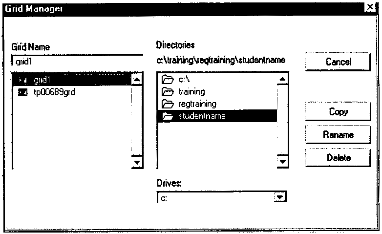
Naming the Grid
The name of "Grid I " does not fit into our naming convention. Ideally, we should be able to rename this using the Grid Manager except ArcView will not allow a grid to be renamed if it has it loaded into memory. So we will make a copy of it instead. We Pull down the File menu and select "Manage Grids..." A pop-up window appears and we select the grid called "Gridl". We click on the "Copy" button and name the new grid (for example: "ddOO689grd") to indicate that the grid is in decimal-degrees format, the number of the T-Sheet, "grd" for a grid file. This will be the grid that we will vectorize using ArcScan.
Vectorization of grids using ArcScan
Beginning the ArcScan Session
ArcTools Menu
Edit Tool Menu
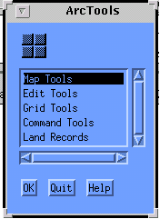
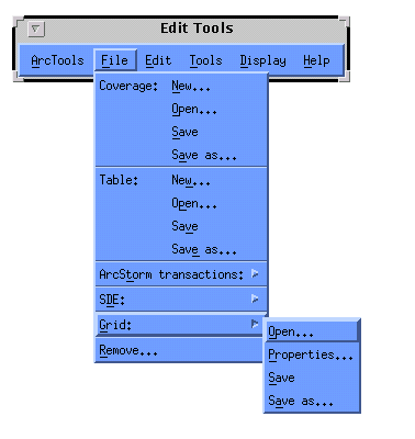
We begin by typing at the main window that appears the command "arc". This will execute the ArcInfo program and the prompt will read "Arc". Now start the ArcTools program by typing the command "ArcTools". This will pop up the graphic window shown above. From the menu bar, select "Edit Tools". A new window will appear that reads "Edit Tools". From the pull down display select File, Grid, and then Open.
Selecting the Grid
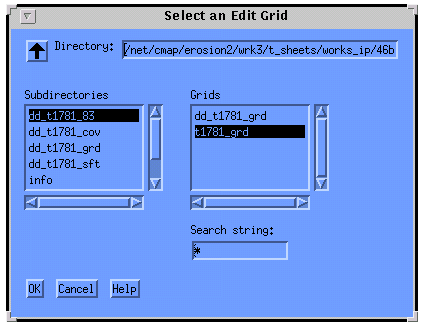
This will open the "Select an Edit Grid" menu from which we can maneuver to the folder we created your workspace for this T-Sheet and pick the Grid you created in the previous ArcView registration Process. Once you select a grid, a map of the Grid will now be draw in the graphic window.
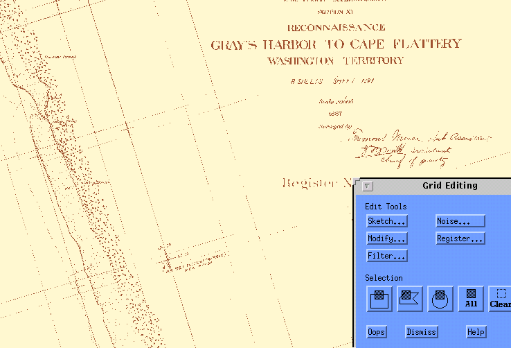
This will be the Grid we will be using in ArcScan. A new window will appear after the map is drawn, that reads "Grid Editing". This set of icons allows the user to cleanup any "noise" found on the scanned image caused by dust, debris, or stray and unwanted line work.
Grid Tools
ArcScan Session
Before we can start to vectorize the grid we have just created, it is necessary to create a new cover to hold the arcs we will be generating. If we try to do this using command line entry, it can become a very cumbersome process that involves generating tics, entering boundaries, and registering. This has already been done in our previous ArcView process, so to take advantage of that, an AML was created called "createnew.aml". This AML takes the min and max values from the grid and uses them to create a boundary file, tics, and set up a .aat table for our coverage codes. When the AML is run it will prompt you for the grid we will be processing, then ask us for the name of the new coverage. I generally give the coverage the same name as the grid with a "_cov" suffix and the end instead of "grd".
Joining our new cover to its associated grid
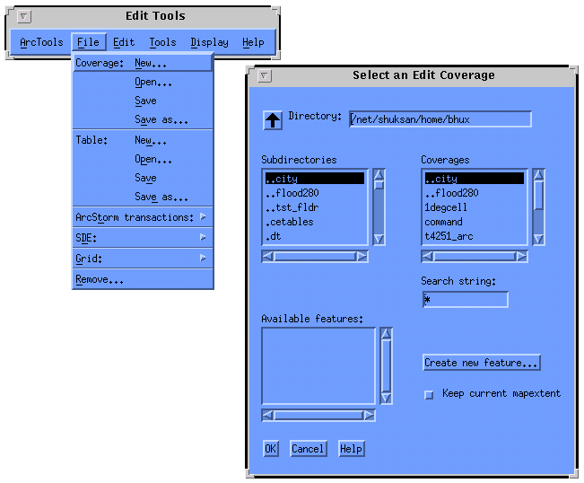
From the Edit Tools menu bar, we pull down the file menu and select "Coverage: open". A new window appears that reads "Select an Edit Coverage". Under the display that reads "Coverages" we select the coverage we just created and under the display that reads "Available Features" click the feature type 'arc". Then click on "OK". The map of the grid begins to redraw, and afterwards, a vector coverage of the new map is drawn on top of the existing grid.
Edit Cover Menu
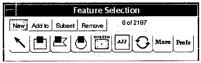
Feature Selection
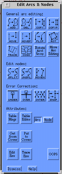
Afterwards, two other windows appear. The first is called "Edit Arcs and Nodes" and it gives a grouping of helpful icons to vectorize (trace) and edit the line work we create. The second window reads "Feature Selection" and it allows us to select the line work we want to perform an edit on.
ArcScan Procedures
From this point on all the procedures used to trace vectors for our new coverage are the same that would be used in a normal ArcEdit session using ArcTools. The exception is that with ArcScan, we also have a trace tool available to us in the "Edit Arcs and Nodes" window.
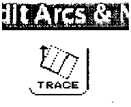
Trace Button
Tracing Operations
The tracing program gives us the ability to determine the direction we want to proceed in vectorizing the line. We can change the direction of the tracer by clicking the right button on our mouse. If we click the right button a few times and you can see how the arrow moves. It's pointing just slightly off of the line, so we can see its direction better. Now, if we were to click both buttons at the same time, the tracing will occur. The tracer stops whenever it encounters another line that intersects it (a junction). At each junction the user has the ability to change the direction of the tracer. We continue proceeding the tracer around the object hat we are vectorizing . If the tracer collected the wrong line at any time, we can move back one junction by typing the number 5 on the keyboard. Below is a listing of the available operations you can use while tracing...
Now Code Your Arcs
The next step is to code all of the arcs that we have vectorized. We want all of the arcs in our coverages to have a Feature Code or "f-code". But we first have to add this field into our Arc Attribute Table (.AAT). This table is a part of the coverage you have created. To begin this process, we click on the Table Manager button located in the "Edit Arcs and Nodes" window. A new popup window appears that allows us to add new items to the existing AAT.
 Table Manager Button
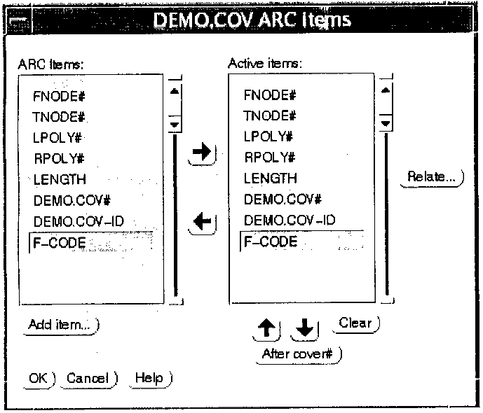 Table Items
Add Items
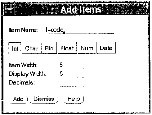
We click on the "Add Item" button within that window and watch as another window appears that allows us to specify "f-code". The item type will be "Int" for integer, and the item "widths and display widths" will both be 5. We click "Add" when we have entered this information. The new item is added to the AAT listing. Now we are ready to assign "f-code" values to the arcs we have captured.
Calculate the f-code
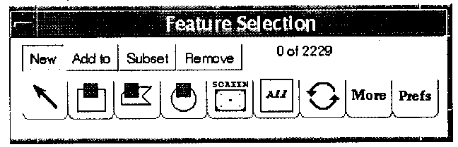 Feature Selection
 Editor Button
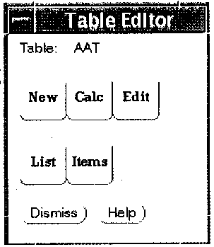
Table Editor
Using the Selection Arrow found in the "Feature Selection" box, we select all of the arcs that we have vectorized. Once we have selected the majority of the arcs, we click on the Table Editor button found on the "Edit Arcs and Nodes" window. A new popup appears that allows us to calculate, edit and list our Arc Attribute AAT Table. We start by looking at the available items in the AAT by clicking on the "Items button". The "f-code" item we added to the AAT is now present at the bottom. Also, the "field widths" and the integer "I" have been added. We quit the window when we are finished.
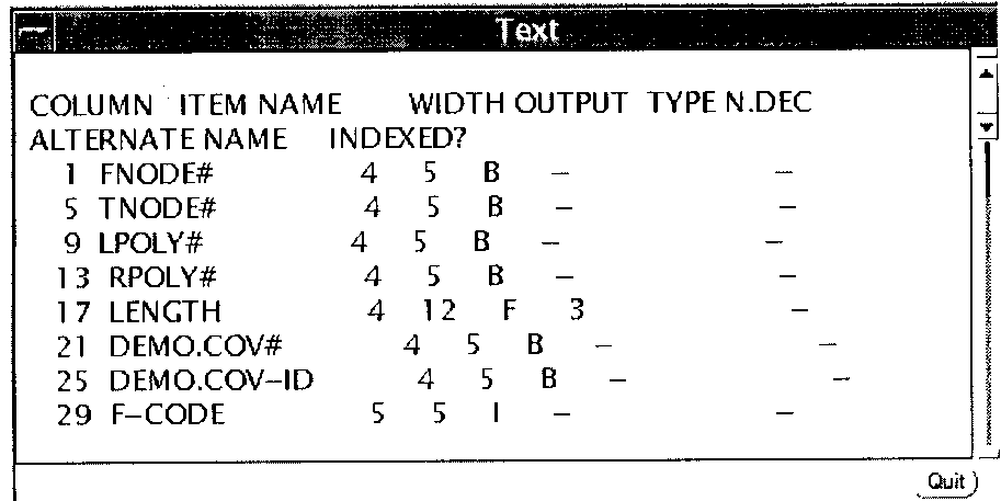 Items List
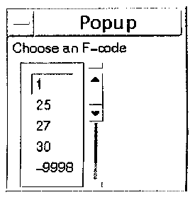 F-Code Popup
Ww now click on the Calc button and see a new popup appear that prompts you for an f-code. The correct code is now put in for the lines selected. The vectorization process is now completed!
Error Analysis
The methodology currently being used by the NOAA data rescue project is to register the scanned map images using the longitude and latitude lines that were drawn on the source maps by the original cartographer and survey teams. These were either in the North American Datum (NAD) (historical maps older than the 1927) or the North American Datum 1927 (NAD27) (contemporary maps). The survey teams also plotted the location of the benchmarks or survey marks used during their fieldwork Some maps contained both, NAD longitude and latitude lines and update marks in NAD27. For the NOAA data rescue project, all maps were converted to the newest datum NAD83 using accepted conversion methods. This was done so maps from different dates could be compared with each other and the NGS benchmarks/survey marks on these maps could be compared with current NGS data sheets.
According to NOS guidelines, map features critical to safe marine navigation are to be mapped to accuracy stricter than national standards. More specifically, the shoreline is mapped to within 0.5 mm of (at map scale) of true position. With a 1:10,000 scale, this is 5.0 m on the ground. Fixed aids to navigation and objects charted as landmarks must be located within 3.0 m at this scale. Because longitude and latitude lines are aids to navigation, the assumption is made that they and the survey markers were drawn on the original map with the same 3.0 m accuracy. If this is correct, then the coordinates of these survey markers can be used to provide an independent check of the accuracy of the registration and data extraction process (Ellis 1978, Shalowitz 1964).
Several sources may introduce error in the final digital data. The primary sources are:
As a test of accuracy of our methodologies, the shoreline and locations of 29 National Geodetic Survey (NGS) survey markers were digitized from eight topographic sheets from mapping project, PH-62, conducted between 1950 and 1951 by the Coast and Geodetic Survey (now the National Ocean Service). The digitizing was done using ArcInfoTM and ArcScanTM software. The ArcScanTM software allowed lines to be digitized to within ˝ the width of what was seen as the raster image of the line or approximately two pixel widths. At 400 dpi resolution for scanned images on a 1:10,000 map, the location of lines was estimated to be within 1.3 m of true.
The markers selected are evenly spread over the entire mapped area and all had sub-meter accuracy. The published location of these same marks were obtained from the NGS and used to create a separate GIS point coverage. These two digital data sets were then overlaid for comparison. (Figure 1)
Trend Analysis of the Extracted Line Work
The accuracy assessments that may be conducted vary based on the number of survey markers that are recovered on a given map and their known positional accuracy. In all cases, calculation of the minimum, mean, and maximum values will give an overall accuracy assessment of the data conversion process if three or more markers are available and they are well distributed over the land portion of the map. If five or more survey marks are recovered, and they are distributed throughout the map, then a trend and skew analysis may be conducted.
The skew analysis may be used to determine if the mean error obtained is skewed toward the minimum or maximum value of the sample. If the sample is skewed to the left (negative), then a majority of the sample values are less than the mean. Conversely, a right (positive) skew indicates that a majority of the values are greater than the mean.
A trend analysis may be conducted to determine if the measured errors (between known coordinates and those derived from the vectorized data) are systematic. Simple linear regression may be used to determine if a linear trend exists in the X or Y coordinate. A systematic error in the X or Y coordinate may be an indicator of errors in the scanning or projection process. For example, variations in roller speed (the speed at which the paper map traveled under the scanning head) during the scanning process may have resulted in a stretch along the Y coordinate that resulted in increased error as one travels from the bottom to the top of the map.An Example Using T-9521
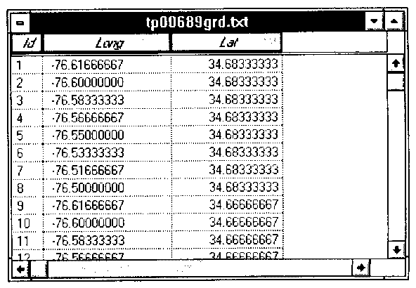
The following example is based on T-sheet T-9521 of Grayland, Washington completed in 1951 at a scale of 1:20,000. This T-sheet was transformed between NAD27 to NAD83 using ArcInfoTM software and the line work on the raster image extracted and saved as lines using the ArcScanTM. Both software packages are from Environmental System Research Institute, Inc., Redlands, California.
During the vectorization process, crosshairs representing the location of survey marks were extracted as lines. The coordinates of the junction of the crosshairs were obtained in ArcEditTM for seven survey markers and compared to published coordinates obtain from the National Geodetic Survey (NGS) for these same markers. An example of a NGS data sheet is contained in the appendix. In Table 1, below, the extracted coordinates are compared with those obtained from the NGS for sheet T-9521.
Table 1. Comparison of published and extracted coordinates for seven survey markers on topographic sheet T-9521. Values are in meters.
|
Marker Name |
PID |
X-Map |
Y-Map |
X-NGS |
Y-NGS |
X Diff |
YDiff |
|
LAST |
SD0046 |
224500.59 |
176397.72 |
224502.58 |
176397.70 |
1.99 |
0.02 |
|
ISLAND |
SD0434 |
228860.78 |
174855.20 |
228858.36 |
174855.21 |
2.42 |
0.01 |
|
BERT |
SD0438 |
227876.19 |
174080.40 |
227879.70 |
174079.37 |
3.51 |
1.03 |
|
DIKE |
SD0443 |
227326.55 |
173952.92 |
227333.32 |
173951.33 |
6.77 |
1.59 |
|
ROBIN |
SD0439 |
227862.80 |
173660.43 |
227865.44 |
173661.49 |
2.64 |
1.06 |
|
GRAY |
SD0054 |
225576.82 |
170529.83 |
225583.41 |
170529.86 |
6.59 |
0.03 |
|
FIRST |
SD0060 |
225756.67 |
166744.23 |
225758.32 |
166745.76 |
1.65 |
1.53 |
|
Minimum |
1.65 |
0.01 |
|||||
|
Mean |
3.65 |
0.75 |
|||||
|
Maximum |
6.77 |
1.59 |
Data sheets with coordinates for NGS and U.S. C&GS survey marks may obtained from the World Wide Web at http://www.ngs.noaa.gov.
Simple Tests
Utilizing the information in Table 1, we determined the minimum, mean, and maximum error associated with sheet T-9521. The standard deviation and median of the X difference and Y difference are 2.14 and 2.64 m and 0.717 and 1.03 m respectively. The Pearsons coefficient of skew may be used to determine if there is a tendency for the values to be larger or smaller than the mean. The formula for this test is as follows:
sk = 3 ( Mean – Median)
Standard Deviation
where sk is the coefficient of skew. Negative values indicate that the scores are negatively skewed toward the sample minimum, a positive skew indicates that the sample is skewed toward the sample maximum. In the above example, sk was 1.4 for the X difference and –7.8 for the Y difference. This indicates that the error in the Y coordinates for this map tend to be less than the mean, while errors in the X coordinates tend to be larger than the mean.
Based on the assumption of a normal distribution, the maximum error (99.87% probability) may be calculated as follows:
Max99.87% = 3 * Standard Deviation + Mean
The XY combined error has a mean value of 3.82 m with a positive skew and a standard deviation of 2.09 m. The error in this T-sheet varies between a low of 1.99 m to a high of 6.95 m, with a 99.87% change that the error is never greater than 10.09 m based on the normal distribution assumption.
Regression Test
In cases where more than five survey markers are available for a given area a linear regression model may be constructed. The model hypothesizes that the actual X or Y coordinate (from the NGS) may be calculated based on the measured values obtained from the T-sheets and a one-dimensional slope factor with a value of one and a intercept value of zero. If this is not true (i.e., the slope factor significantly varies from one) then a systematic error may be present in the given dimension. For this example the following equation for a line is fitted to the data:
X actual = X measured * m + b
where m is the slope of the line and b is the y intercept. In a case where no linear systematic error exists, the m value would be equal to one and b would be equal zero. If the calculated m is significantly different from one then there is a systematic error in the given coordinate. If the b value is significantly different from zero, then the entire map may be offset from its origin by the given amount.
The regression statistics calculated for the X and Y coordinates, shown in Table 1, are presented in Tables 2 and 3.
Table 2. Linear regression results for the X coordinates for topographic sheet T-9521. Regression Statistics Multiple R 0.999998181 R Square 0.999996363 Adjusted R Square 0.999995635 Standard Error 3.265780195 Observations 7 Coefficients Standard Error t Stat P-value Lower 95% Upper 95% Intercept 152.4071158 193.3383425 0.788292244 0.46623804 -344.5841 649.3983 X Variable 1 0.999341135 0.000852358 1172.442494 8.5673E-15 0.99715 1.001532
Table 3. Linear regression results for the Y coordinates for topographic sheet T-9521. Regression Statistics Multiple R 0.999999961 R Square 0.999999922 Adjusted R Square 0.999999906 Standard Error 0.989762683 Observations 7 Coefficients Standard Error t Stat P-value Lower 95% Upper 95% Intercept 32.07702253 21.62275831 1.483484303 0.19805905 -23.50596 87.66 X Variable 1 0.999814456 0.000125049 7995.394051 5.809E-19 0.999493 1.000136
The m and b values for Table 2 are 0.999 and 152.4 m, respectively. The standard error estimate of b is 193 m. In Table 3 the m value is 0.999 and b is 32 m with a standard error estimate of 21 m. These values indicate that the measured X and Y coordinates for T-9521 do not have a significant offset in the X or Y origin. The closeness of both m values to 1 show that a linear systematic error is not evident in the data.
To provide an example of how a systematic error would affect the results, the measured X coordinates shown in Table 1 were modified. By adding 15 m to the X coordinate value of each survey marker for every 1000 m the marker was west of survey marker "LAST" (the east most survey marker in the table), a linear systematic error was introduced into the measured X coordinates (i.e., the error increased by 15 m for every 1000 m traveled west).
The linear regression analysis was then repeated for the X coordinate using the modified data. The calculated m was 0.980 and the b, or intercept, was 4516.6 m with a standard error of 1769.0 m. Thus, when a systematic error was introduced the m value became less than 0.99 and the standard error of the b constant became much smaller than the b value itself.
Overall Error Assessment for Project PH-62
A given NOAA survey project is conducted over a one to three year period and may involve from one to many individual T-sheets. Since the same personnel work on a project throughout its lifetime it can be assumed that the same (or similar) procedures were followed for construction of the T-sheets. Based on this assumption, an error assessment may be made for a project as a whole, as well as for individual T-sheets. Combining information allows for a more robust analysis to be conducted, as the sample size (i.e., number of survey markers utilized) will increase.
For PH-62, the mean, standard deviation and median were calculated (Table 4 next page) for differences in X, Y, and XY. For XY mean is 3.06 m (10 ft) with a positive skew (1.35) and the standard deviation is 1.48 m. Based on the normal distribution assumption, the error in this project varied between 0.25 m to 6.95 m, with a 99.87% chance that the error is less than 8.30 m.
Table 4. Comparison of published and extracted coordinates for PH-62 Marker Name Sheet X-Map Y-Map X-NGS Y-NGS X Difference Y Difference XY Difference BURNT T-10344 223964.43 110011.55 223963.64 110008.83 0.79 2.72 2.83 McKENZIE HEAD T-10344 225360.68 111869.24 225361.94 111866.35 1.26 2.89 3.15 DEADMAN T-10344 224599.66 112231.37 224603.96 112228.90 4.30 2.47 4.96 NORTH HEAD LH 1909 T-10344 224448.75 113573.92 224449.87 113572.27 1.12 1.65 1.99 BAKER WEST BASE T-10340 229465.08 115093.09 229468.01 115091.62 2.93 1.47 3.28 LAKE T-10340 227257.22 115176.20 227256.29 115172.97 0.93 3.23 3.36 TURN T-10340 226915.97 116245.84 226914.31 116242.69 1.66 3.15 3.56 APEX T-10340 230253.14 118727.98 230256.05 118726.66 2.91 1.32 3.20 TIOGA RESET T-10340 226500.91 120421.00 226497.76 120419.81 3.15 1.19 3.37 BONNIE T-10649 226749.26 123517.93 226748.93 123516.53 0.33 1.40 1.44 GREEN RESET T-10649 226899.68 127530.55 226897.84 127528.75 1.84 1.80 2.57 SNAKE 2 T-10649 229550.84 128681.48 229546.62 128682.10 4.22 0.62 4.27 DOANE 2 T-9637S 229554.55 137083.37 229555.82 137082.62 1.27 0.75 1.47 OYSTER 2 T-9637S 227160.89 141168.77 227158.61 141171.03 2.28 2.26 3.21 GOULTER 2 T-9637S 229760.29 141539.65 229758.58 141538.88 1.71 0.77 1.88 MESS T-9637N 229982.42 144909.53 229983.85 144910.32 1.43 0.79 1.63 BETTER T-9637N 228653.27 147710.59 228649.96 147713.08 3.31 2.49 4.14 GRASSY 1939 T-9634S 228954.83 150373.61 228953.86 150377.30 0.97 3.69 3.82 LEAD 4 T-9634S 228196.88 151487.00 228196.31 151490.99 0.57 3.99 4.03 WILLAPA BAY LIGHT T-9634N 226814.61 160922.42 226814.73 160922.64 0.12 0.22 0.25 LARKIN T-9634N 228934.47 162353.00 228935.28 162353.30 0.81 0.30 0.86 BEACH 2 T-9634N 225942.13 163121.74 225942.72 163124.39 0.59 2.65 2.71 FIRST T-9521 225758.32 166745.76 225756.67 166744.23 1.65 1.53 2.25 GRAY T-9521 225583.41 170529.86 225576.82 170529.83 6.59 0.03 6.59 ROBIN 1940 T-9521 227865.44 173661.49 227862.80 173660.43 2.64 1.06 2.84 DIKE T-9521 227333.32 173951.33 227326.55 173952.92 6.77 1.59 6.95 BERT 1940 T-9521 227879.70 174079.37 227876.19 174080.40 3.51 1.03 3.66 ISLAND T-9521 228858.36 174855.21 228860.78 174855.20 2.42 0.01 2.42 LAST T-9521 224502.58 176397.70 224500.59 176397.72 1.99 0.02 1.99 Mean 2.21 1.62 3.06 Standard Deviation 1.67 1.14 1.48 Median 1.71 1.47 3.15 Minimum 0.12 0.01 0.25 Maximum 6.77 3.99 6.95 Error Analysis Conclusions The process of converting the raster data to vectors is a multi-step process. Each step, or the quality of the original data source, may introduce error into the final digitized data. The conversion process herein utilized the existing longitude and latitude coordinate system on the map. Thus, to obtain an independent assessment of the error within the final data product a method was needed that could compare measured (i.e., from the digitized data) and published coordinates for known points on the map. The preceding examples demonstrate how the coordinates for survey markers, published by National Geodetic Survey, may be used in combination with coordinates measured from the vectorized T-sheets to obtain error assessments for the map conversion process. The statistical methods described here may be used to identify linear and systematic errors in the vectorized data. These statistical methods are simple and may be conducted using the data analysis tools available in most computer spreadsheets (e.g., Lotus 1-2-3TM or ExcelTM). The following conclusions can be made about the methodologies and procedures used in this data conversion process:
This research would not have been possible without the tremendous support of many individuals involved directly and indirectly in the project. Gregg Fromm NOAA, Silver Spring, MD Project concept and direction Ron Travis and Mike McGinley NOAA, Silver Spring, MD Data Scanning David McKinnie and Linda Maxim NOAA, Sand Point, WA West Coast NOAA support Cindy Fowler Coastal Services Center, SC Project Development Michael D. Rink Coastal Services Center, SC Training, Training Manuals, etc Jeff Cowen Coastal Services Center, SC Computer Programming /Support Richard C. Daniels Dept. of Ecology, WA GIS and Statistical Analysis George Kaminsky Dept. of Ecology, WA Project Management and Suport
Anders, F.J. and Byrnes, M.R. 1991. Accuracy of Shoreline Change Rates as Determined from Maps and Aerial Photographs. Shore and Beach, Vol. 59, pp. 17-26. Byrnes, M.R., Hiland, M.W., McBride, R.A., and Westphal, K.A. 1991. Pilot Erosion Rate Data Study: Harrison County, Mississippi. Federal Emergency Management Administration, Office of Risk Assessment, Washington, DC. Ellis, M.Y. (editor). 1978. Coastal Mapping Handbook. U.S. Department of Commerce, National Ocean Survey, Washington, DC. Schalowitz, A.L. 1964. Shoreline and Sea Boundaries, Volume 2. U.S. Department of Commerce, Coast and Geodetic Survey, Washington, DC. Michael D. Rink. 1997. Procedures for the Registration and Vectorization of NOS T-Sheets, Version 2.0, pp. 1-49.
Robert H. Huxford, Richard C. Daniels
Acknowledgments
References
Coastal Monitoring and Analysis Program
P.O. Box 47600
Olympia, WA 98504-7600
Phone: (360) 407-6780
E-Mail: bhux461@ecy.wa.gov
Fax (360) 407-6535