CONVERTING POINT ESTIMATES OF DAILY RAINFALL ONTO A RECTANGULAR GRID
Steven D Lynch
Department of Agricultural Engineering
University of Natal
Pietermaritzburg, 3209
South Africa
Rainfall measurements are commonly observed at point locations and these values are required inter alia by Hydrologists and Engineers to be converted to a raster format. The most common method that is used is the inverse distance weighting interpolation technique. This technique uses the location and magnitude of the rainfall to determine estimates of rainfall at unmeasured locations.
South Africa occupies an areal extent of approximately one million square kilometres. Daily rainfall is measured, in real-time using telemetry, at approximately 170 locations in South Africa and at a further 1,900 locations daily that are then assimilated monthly into a national daily rainfall database by the South African Weather Bureau.
Areal estimates of daily rainfall are of paramount importance especially in water-poor countries such as South Africa. Researchers often require that an estimate of rainfall at ungauged points are determined in order for them to assess the spatial distribution of the rainfall amounts.
The techniques, using the ArcInfo GIS, will be discussed in this paper to assist researchers in converting point estimates of daily rainfall to a raster surface that can be used to describe the daily rainfall in an areal context.
INTRODUCTION
The South African Weather Bureau (SAWB) has approximately 170 automatic weather stations that relay inter alia daily rainfall amounts to their central computer each day. On the other hand, there are approximately 1900 active rain-gauges that are used to collect rainfall amounts over South Africa. These daily data are collated by the SAWB at the end of each month and are then checked for possible errors (Lynch, et al., 1996). Researchers wanting to obtain current daily rainfall data are therefore required to wait a few months before the data becomes available and then these data are not current anymore. The author requested, in February 1998, from the SAWB the complete daily rainfall database for November 1997 and was supplied with the daily rainfall amounts for approximately 800 stations which relates to about 42% of the complete database. Research presented in this paper will examine some techniques that can be used to convert the automatic weather station data, which are available on the same day, to estimates of daily rainfall amounts at the sites where rainfall is measured daily but data only become available a few months hence. These estimates can be replaced by the more detailed daily rainfall values once they become available from the SAWB.
LOCATION AND METHODOLOGY
The SAWB agreed in October 1997 to supply the Department of Agricultural Engineering at the University of Natal in Pietermaritzburg with their synoptic data on a daily basis via an X25 dial-up facility. The author has decided to use the daily rainfall data derived from the synoptic data received on the 16th of November 1997. Reasons for choosing this date include inter alia the following; synoptic data from the approximately 170 automatic weather stations are available, a reasonable number of the daily rainfall weather stations data received by the SAWB have been processed by them are available and that the spatial complexity of the distribution daily rainfall over South Africa are displayed on this day.
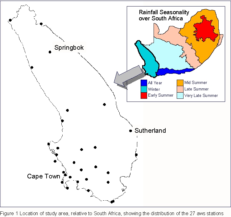
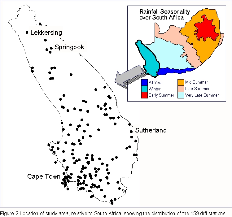
There are 27 automatic weather stations (aws) in the winter rainfall region of South Africa, as delineated in Schulze (1997), Fig. 1, and 159 daily rainfall (drfl) stations had been processed for the same area, Fig. 2, by the SAWB when this research was initiated in February 1998. Different spatial interpolation and regression techniques will be examined in this research to use the 27 automatic weather stations information to predict daily rainfall amounts at the 159 positions that record rainfall on the same day. The rationale behind this research is that aws data can be accessed in real-time and on the day that the measurements are made. The spatial density of these data are much coarser than the spatial density of the entire SAWB daily rain-gauge network. Unfortunately the drfl data only become available at a much later date. This project will be using historical aws data, for 16 November 1997, and aspire to produce the daily rainfall amounts that are reflected in the drfl data which have a much finer spatial resolution. In other words, spatial interpolation techniques will be used to try and mimic the data reflected by the drfl data that are received many months hence.
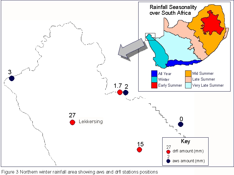
The dilemma that we are faced with can be illustrated using an area, approximately 15,000km2 in size, in the northern section of the study area, Fig. 3. The maximum aws amount is 3mm and the maximum drfl amount is 27mm. The question that then comes to mind is, how do you interpolate values of 0, 2 and 3mm to give a value of 27mm ?. An interpolation method that uses more than just the properties of the surrounding data points is therefore required.
METHODS OF SPATIAL INTERPOLATION AND REGRESSION
The procedure of estimating the value of properties at un-sampled sites within the area covered by existing point observations is called interpolation. The value of a property between data points can be interpolated only by fitting some plausible model of variation to the values at the data points and then calculating the value at the desired location. The problem of interpolation is thus a problem of choosing a plausible model to suit the data (Burrough, 1986).
INVERSE DISTANCE WEIGHTING METHOD
In this method weights are calculated depending on the distances between the location where an estimate is required and the location where the rainfall are measured. Because moving average methods such as inverse distance weighting are by definition smoothing techniques, the maximum and minimum values can only occur at the measured points. This technique will therefore never produce a value that is higher than the maximum value in the observed data set. The fact that daily rainfall amounts are often confined to a small area causes another problem when using this type of interpolation as rainfall amounts are generated for areas where no rain fell. These amounts do however decrease with distance but there is not a sufficient spatial density of rain-gauges to explain this.
SCHÄFER DAILY RAINFALL ESTIMATION METHOD
Raster median monthly precipitation (MMP) surfaces have been developed for South Africa at a spatial resolution of 1 minute by 1 minute of a degree (Dent, et al., 1988). The Schäfer daily rainfall estimation method (Schäfer, 1991) firstly expresses the daily rainfall at each measured site as a ratio of the MMP, where the month equals the month that the daily values were measured, at that position. An interpolation method is then used to convert these point values onto a raster surface at the same spatial resolution as the MMP. Finally this surface is multiplied by the MMP surface to yield a daily rainfall surface for a particular day. The main disadvantage of this method is that an assumption has been made to the effect that the distribution of daily rainfall amounts are similar to the distribution of the mean annual precipitation over South Africa.
MULTIPLE REGRESSION METHOD
Multiple regression techniques have successfully been used in the past to describe the spatial distribution of mean annual precipitation over South Africa (Dent, et al., 1988). Regression techniques require that the spatial density of the locations at which the values are observed is sufficient to explain the variation in the measured amounts. This technique is prone to extrapolate the estimated values to below the minimum and above the maximum of the observed points and in some cases negative rainfall amounts are predicted.
SPLINE INTERPOLATION METHOD
The spline mathematical functions are akin to the flexible ruler that was historically used to produce a smooth curve when joining a set of points. Spline functions can produce estimates that are above and below the measured minimum and maximum values. This is not always desired as maxima and minima values are often produced where they do not occur in nature.
KRIGING INTERPOLATION METHOD
Kriging uses the covariance structure of the field to estimate interpolated values. The resulting interpolated field is optimal in the sense of minimizing the variance among all possible linear, unbiased estimates. Kriging requires a two-step process - the fitting of a semi-variogram model function (of distance) followed by the solution of a set of matrix equations.
INTERPRETATION OF THE RESULTS
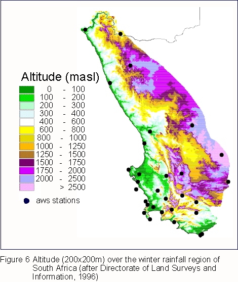
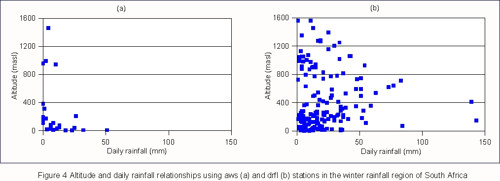
It is generally accepted that altitude is the main variable governing the spatial distribution of rainfall in areas of complex topography (Sevruk, 1997). The area that has been selected for this research project has a complex topography (Table 1 and Fig. 6) but the daily rainfall amounts for the aws and drfl sites are not correlated with the altitude values, Fig. 4a and Fig. 4b, respectively, in any way.
Table 1 Altitude and daily rainfall statistics for the study area
|
Statistic |
Altitude (masl) |
Daily rainfall (mm) | |
| aws | drfl | ||
| Minimum | 0 | 0.0 | 0.0 |
| Maximum | 2192 | 51.0 | 143.0 |
| Mean | 575 | 10.9 | 22.6 |
| CV (%) | 68 | 111.9 | 97.2 |
| Median | 533 | 8.0 | 17.0 |
| Sample size | 148483 km2 | 27 | 159 |
The term random can be described to imply, without method or conscious choice, with equal chances for each item or without aim or purpose or principle (Tulloch, 1993). Perusal of the distribution amounts of the daily rainfall presented in this research has led the author to believe that there is no measurable explanation as to how much rain is precipitated at a given location and could therefore be a random amount. This might be explained by a verse from The General Epistle of James, Chapter 5 verse 18, which reads, "And he prayed again, and the heaven gave rain, and the earth brought forth her fruit." (Holy Bible, 1968).
The problem mentioned in Fig. 3 and the fact that the given set of daily rainfall data, i.e. the aws dataset, do not contain any values above 51mm whereas the data received a few months hence do have daily rainfall amounts well in excess of 51mm. The inverse distance weighting method does not have the ability to predict values above the maximum rainfall amount given in the input dataset. The spline method, on the other hand, can produce values well in excess of the input maximum values under certain circumstances.
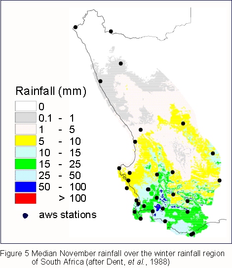
The Schäfer daily rainfall estimation method, the multiple regression method and the Kriging method can theoretically produce predicted values that are higher than those found in the input dataset. The median monthly rainfall surface, Fig. 5, does not show any rainfall variation in the area described in Fig. 3 and the Schäfer daily rainfall estimation method therefore cannot produce the required amount of 27mm. Perusal of the 200m by 200m spatial resolution altitude surface (Directorate of Land Surveys and Information, 1996), Fig. 6, does however, illustrate that topographic variation exists in the area surrounding the 27mm rain-gauge in question. Unfortunately no correlation exists between the rest of the aws stations, or any of the drfl stations, and altitude. Surfaces that include inter alia altitude, distance from the sea and surface roughness have been used in a multiple regression process and have failed to yield any significant goodness of fit statistics (r2a = 0.19 , n=27).
The 27 aws stations were used as input to the different interpolation and regression techniques and the statistics of the predicted values at the 159 drfl positions are displayed in Table 2. Perusal of Table 2 would suggest that the Schäfer daily rainfall estimation method is the most suitable for the estimation of a daily rainfall surface for the winter rainfall region of South Africa on 16 November 1997. The Group_20 and Group_33 statistics are described in Lynch, et al. (1995) and are calculated as follows. For each of the 159 points a counter is used to record the number of times that the interpolated or regressed estimate is within �20% or within �30% of the drfl value at that position. The final count is then expressed as a percentage of the total number of points (i.e. 159). The Schäfer daily rainfall estimation method, for example, produces estimates of the daily rainfall that are within �20% of the true values at 11.9% of the drfl stations (Table 2). The classic statistics of inter alia mean, minimum, maximum and standard deviation do not lend them to the comparison of raster surfaces as can be seen if one had to compare a surface to a mirror image of that same surface, the classic statistics would be the same indicating that the surfaces are the same.
Table 2 Goodness of fit statistics when aws data are used to predict the drfl data at the 159 points
| Statistic | drfl | IDW* | Schäfer | Regression | Spline | Kriging |
| Min (mm) | 0 | 0 | 0 | -9.5 | -21.1 | -1.6 |
| Max (mm) | 143 | 50 | 95 | 56 | 53 | 43 |
| Sum (mm) | 3591 | 1548 | 2056 | 1801 | 1284 | 1320 |
| Mean (mm) | 22.6 | 9.7 | 12.9 | 11.3 | 8.1 | 8.3 |
| Std deviation (mm) | 21.9 | 10.9 | 18.5 | 10.9 | 13.9 | 11.0 |
| Correlation with drfl | 0.17 | 0.24 | 0.46 | 0.06 | 0.14 | |
| RMSE* (mm) | 26.1 | 26.8 | 22.5 | 29.1 | 27.0 | |
| Mean residual (mm) | 12.6 | 9.4 | 11.0 | 14.2 | 13.9 | |
| F-statistic | 4.08 | 1.41 | 4.07 | 2.50 | 4.00 | |
| Group_20 (%) | 9.4 | 11.9 | 6.3 | 8.8 | 8.8 | |
| Group_33 (%) | 13.8 | 15.1 | 18.2 | 11.9 | 13.8 | |
| Sample size | 159 | 159 | 159 | 159 | 159 | 159 |
| *inverse distance weighting | *root mean square error | |||||
A discriminant analysis (SAS, 1996; Dicks, 1998) was performed on the regression variables to determine whether the classification into the winter rainfall region is acceptable or not. The input variables included for each of the drfl stations on 16 November 1997, the rainfall amount, the MMP of November, the altitude, a surface roughness index, the distance from the sea, the latitude and longitude and the class variable was the seasonality region that each point fell into.
Table 3 Discriminant analysis describing the percentage of observations that were grouped into each of the seasonality regions
|
Region |
Percent classified into region |
| All Year | 99 |
| Early Summer | 88 |
| Late Summer | 97 |
| Mid Summer | 76 |
| Very Late Summer | 93 |
| Winter | 94 |
The results from the discriminant analysis , Table 3, show that 94% of the drfl stations are classified to be within the winter rainfall region of South Africa as described in Schulze (1997). The 6% that were mis-classified fell either into the all year or the very late summer regions which are adjacent to the winter rainfall region.
DISCUSSION AND CONCLUSIONS
The bad news is that a GIS user cannot simply throw their data into the first available interpolation method and hope to get a swift and satisfactory solution (Hu, 1995). When converting point rainfall estimates onto a raster surface one needs to know why this conversion is necessary. If the predicted values at ungauged sites are required for further use in a modelling exercise then a particular interpolation approach might be used. On the other hand, however, if the predicted surface is to be portrayed in a map then in order to present a useful and truthful picture, an accurate map must also tell white lies (Monmonier, 1996), and another method could be used.
The question as to which interpolation or regression technique should be used for converting point estimates of daily rainfall onto a rectangular grid is a difficult one to answer. If the maximum amount of rainfall for the day in question is contained in the input dataset then the inverse distance weighting method can be used. The spline interpolation and the regression techniques should not be used at all as they can produce gross under or over estimates of the daily rainfall at ungauged positions. The Kriging method involves an enormous amount of semi-variogram estimation that does not produce better estimates of the daily rainfall surfaces. The Schäfer daily rainfall estimation method should be used when the input dataset does not contain the maximum rainfall amount on the day in question. The author would therefore recommend that either the Schäfer daily rainfall estimation method, if raster surfaces of median monthly rainfall are available, or the inverse distance weighting method be used when trying to convert point daily rainfall measurements to values at ungauged positions.
ACKNOWLEDGEMENTS
The Computing Centre for Water Research (CCWR) is acknowledged gratefully for their assistance in making this research possible and for allowing the author to make use of their WWW server to publish and disseminate his published articles to the scientific community all over the World. The Research Fund of the University of Natal is thanked for their financial support in this project. The Water Research Commission is also acknowledged for allowing time to do this research. Finally, the South African Weather Bureau is thanked for making their rainfall and synoptic data available.
DISCLAIMER
The information provided herein is subject to change without notice. In no event will I be liable for damages, including loss of revenue, loss of profits or other incidental or consequential damages arising out of the use of or inability to use the information presented in this document. The views contained in this document are my own and are not necessarily the views of the University of Natal.
REFERENCES
Burrough, PA, 1986: Principles of Geographical Information Systems for Land Resources Assessment. Clarendon Press, Oxford, UK.
Dent, MC, Lynch, SD and Schulze, RE, 1988: Mapping Mean Annual and Other Rainfall Statistics over Southern Africa. Univ. of Natal, Dept. Agric. Eng., ACRU Report 27, Water Research Commission, Pretoria, South Africa. Report No 109/1/89.
Dicks, HM, 1998: Personal communication. Dept. Statistics and Biometry, Univ. of Natal, Pietermaritzburg, South Africa.
Directorate of Land Surveys and Information (DLSI), 1996. Private Bag X10, Mowbray, South Africa.
Holy Bible, 1968:King James Version, The British and Foreign Bible Society, London, UK.
Hu, J, 1995: Methods of Generating Surfaces in Environmental GIS Applications. Proc. 1995 Esri User Conference, Palm Springs, CA, USA.
Lynch, SD, Lecler, NL. and Schulze, RE., 1996: Using Real-time Hydrological Data. http://www.ccwr.ac.za/~lynch2/p307.html
Lynch, SD. and Schulze, RE., 1995: Techniques for Estimating Areal Daily Rainfall. Proc. 1995 Esri User Conference, Palm Springs, CA, USA.
Monmonier, M, 1996: How to Lie with Maps. The University of Chicago Press, Chicago, IL, USA.
SAS, 1996: SAS User's Guide: Statistics. SAS Institute Inc., PO Box 8000, Cary, NC, USA.
Schäfer, NW, 1991: Modelling the Areal Distribution of Daily Rainfall. Unpubl. M.Sc.Eng. dissertation, Dept. Agric. Eng., Univ. of Natal, Pietermaritzburg, South Africa.
Schulze, RE, 1997: South African Atlas of Agrohydrology and -Climatology. Water Research Commission, Pretoria, South Africa. Report No TT82/96
Sevruk, B, 1997: Regional Dependency of Precipitation-Altitude Relationship in the Swiss Alps. Climatic Change 36: pp 355-369. Kluwer Academic Publishers, The Netherlands.
Tulloch, S, 1993: The Reader's Digest Oxford Complete Wordfinder. The Reader's Digest Association Ltd., London, UK.